

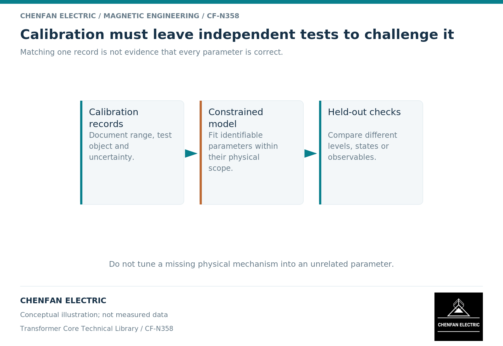
Calibrating a core model to one test is not the same as validating its predictive behavior. Several combinations of material, geometry and circuit parameters can reproduce one observation. The model needs separate checks that challenge the mechanisms it will use in the intended operating cases.
Choose parameters that have physical meaning
Before fitting, identify which parameters are measured, which are design-derived and which are adjustable. Avoid allowing every uncertain quantity to move freely until the residual is small.
A terminal current can be influenced by the magnetizing characteristic, leakage circuit, losses and initial state. Transformer-model guidance demonstrates that even branch placement can affect nonlinear behavior. [1] A fit can therefore compensate for an incorrect model structure by distorting another parameter.
Keep geometric quantities tied to the drawing where possible. A fitted “effective gap” may be a useful lumped parameter, but should not be reported as a measured physical gap unless that interpretation has been established.
Use more than one observable
Matching one root-mean-square current value is weaker evidence than matching the relevant waveform, phase relation and loss over several excitation levels. Select observables that constrain different parts of the model.
For example, a low-level excitation case can constrain one part of the characteristic, while a higher-level case tests the nonlinear region. A connection change can challenge the represented magnetic coupling. A different waveform can challenge history or rate dependence.
Material-model choice sets what behavior the parameters can represent. [2] No amount of fitting can make a memoryless curve reproduce every remanence history without additional state information.
Reserve independent cases before fitting
Divide the available evidence into calibration and validation sets. The validation cases should be relevant but not merely duplicates of the calibration point. Preserve the division before looking at the final fit to avoid repeatedly selecting only favorable comparisons.
An illustrative review might fit a model using two centered excitation levels, then test it against a third level and a different permitted connection. This is a study design example, not a claim that those tests have been performed.
If the model is revised after a validation failure, record the revision and retain a genuinely independent check where possible. Repeated tuning against the same “validation” case gradually turns it into calibration data.
Report residual patterns and uncertainty
| Result pattern | Possible issue to investigate |
|---|---|
| Correct amplitude, wrong phase | Loss or circuit representation |
| Good low-level fit, poor high-level fit | Nonlinear curve range or extrapolation |
| One connection fits, another fails | Coupling or topology representation |
| First cycle fits, later decay fails | Initial state, damping or dynamic model |
| Several parameter sets fit equally | Limited identifiability |
These are diagnostic directions, not automatic fault assignments. The point is to examine structured disagreement rather than compressing every comparison into one average error number.
The handover should include parameter bounds, fitting objective, datasets used, independent results and the range of intended use. Report sensitivity to poorly identified parameters when it affects the decision.
A credible conclusion states what the model predicts beyond the observations used to tune it. It does not claim universal accuracy from one matched test, and it does not convert a fitted parameter into a manufacturing acceptance limit without a separate technical basis.
References
[1] Manitoba Hydro International / PSCAD. The Classical Approach.
[2] Cesare Tozzo / COMSOL. Modeling Ferromagnetic Materials in COMSOL Multiphysics.