

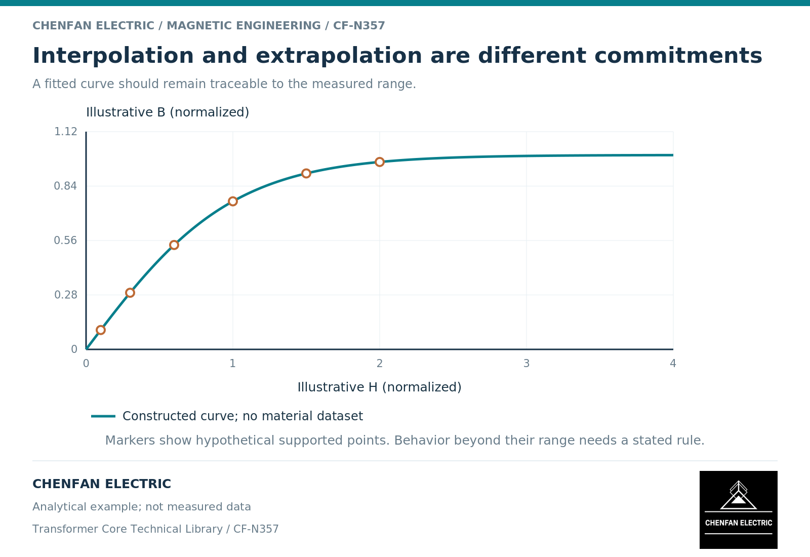
Measured B-H points do not become a reliable simulation input merely by being imported successfully. Interpolation determines the curve between points; extrapolation determines behavior beyond them. Both can materially affect saturation predictions, especially when the available data are sparse near a rapidly changing slope.
Identify the kind of curve being imported
A normal magnetization curve, an anhysteretic relation and a branch of a hysteresis loop are different datasets. Confirm which one the solver expects. A time-ordered loop should not be forced into a single-valued relation by sorting away its history.
Also verify units, axis definitions, material direction, temperature and specimen condition. Field strength in amperes per metre is not magnetomotive force in ampere-turns, and flux density in tesla is not total flux in webers.
Constitutive-model guidance distinguishes these material representations and their intended uses. [1] That distinction comes before choosing a smooth interpolation method.
Inspect the fitted curve, not only the original points
A high-order interpolant can overshoot between sparse points or create an unintended local slope. Smoothing can remove numerical difficulties while also changing the measured characteristic.
The finite-element manual provides a concrete example: its documented B-H handling uses interpolation and may smooth problematic data, while values beyond the supplied range are extrapolated. [2] The engineering lesson is to inspect the curve actually used by the solver rather than assuming it is identical to the source table.
Plot the imported points and implemented curve on the same axes. Examine the low-field region, knee region and highest supplied field. Where the study depends on differential behavior, inspect the slope as well as the curve value.
Mark the boundary between interpolation and extrapolation
The maximum measured B or H should be visible in the model report. Then identify which operating regions exceed it. A small part of the geometry entering an unsupported range can still control a local loss or transient current result.
Do not extend the final measured slope indefinitely without assessing its physical plausibility. Conversely, do not append invented high-field points solely to obtain a desired current peak. Any extension needs an identified theoretical, measured or justified modeling basis.
An illustrative data review can classify each operating point as inside the measured range, near its edge or outside it. This classification is often more informative than reporting a fit error averaged across many low-field points while the critical high-field region is unsupported.
Preserve a traceable material-data chain
| File or record | Purpose |
|---|---|
| Original laboratory data | Preserves measured values and conditions |
| Processed curve | Documents unit conversion, filtering and selection |
| Solver implementation | Shows interpolation and extrapolation behavior |
| Operating-range overlay | Identifies where the model uses unsupported extension |
| Validation cases | Checks the resulting response independently |
A change in the curve-processing method should receive a new model revision. Otherwise two engineers can use the same source dataset and unknowingly calculate with different constitutive behavior.
The final handover should state the supported range and the consequences of any extension. A precise simulation result beyond that range remains conditional, no matter how smoothly the solver converges. Keeping the data boundary visible prevents a material table from being treated as unlimited evidence for every saturation study.
References
[1] Cesare Tozzo / COMSOL. Modeling Ferromagnetic Materials in COMSOL Multiphysics.
[2] David Meeker. Finite Element Method Magnetics User Manual.