

A transfer calculation uses the breaker’s average closing time. The actual operation arrives earlier or later. If the bus is slipping rapidly, that difference can move closure outside the assessed phase window even though the average prediction is correct. [1]
Closing-time evidence should describe a population and its conditions. A single successful timing measurement does not establish the range after temperature, control voltage or mechanism condition changes.
Define the timing endpoints
Record whether delay begins at relay output, coil energization or another reference. Record whether it ends at main-contact closure or an auxiliary indication. Those endpoints can differ. A delay fitted to one boundary cannot be used for another without an established relationship.
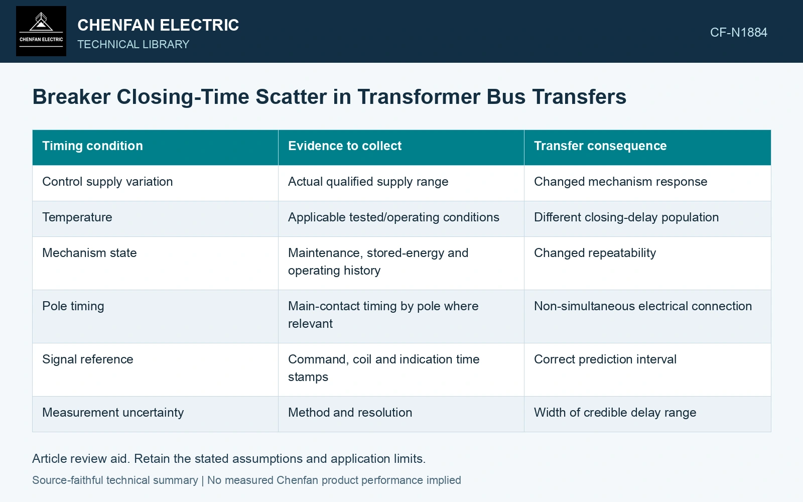
| Timing condition | Evidence to collect | Transfer consequence |
|---|---|---|
| Control supply variation | Actual qualified supply range | Changed mechanism response |
| Temperature | Applicable tested/operating conditions | Different closing-delay population |
| Mechanism state | Maintenance, stored-energy and operating history | Changed repeatability |
| Pole timing | Main-contact timing by pole where relevant | Non-simultaneous electrical connection |
| Signal reference | Command, coil and indication time stamps | Correct prediction interval |
| Measurement uncertainty | Method and resolution | Width of credible delay range |
Translate delay uncertainty into angle uncertainty
Over an interval with nearly constant relative frequency Δf in hertz, a timing error Δt in seconds produces an angle error approximately 2πΔfΔt in radians. This illustration assumes a locally constant slip. Changing slip adds another term and may require the dynamic trajectory.
The formula shows why the same timing scatter matters more in a faster-slip state. It does not provide a permitted angle or a safe delay. Those limits need the accepted motor and mechanical assessment.
Keep tails and correlations visible
Do not assume closing times are normally distributed because a spreadsheet offers a standard deviation. Retain observed extremes, sample conditions and the basis for any extrapolation. A small sample from one warm, healthy mechanism cannot establish every cold or low-control-voltage event.
Delay can correlate with other adverse conditions. A disturbance that lowers control voltage may also alter the motor-bus state. Assess credible combined cases rather than combining uncertainties as though they always occur independently.
Keep measurement uncertainty separate from the observed mechanism population. When quantified uncertainties are combined, use the appropriate sensitivity and correlation information; a bounded delay range is not automatically a standard deviation. [2]
Convert the delay band into an angle band
Assume locally constant slip of 2 Hz and closing-delay uncertainty of ±10 ms. The associated arrival-angle uncertainty is ±360 × 2 × 0.010 = ±7.2°. At 4 Hz it becomes ±14.4°. Use the band in the accepted dynamic case; the mean closing time alone discards this dependence.
References
- P. Muralimanohar, D. Haas, J. R. McClanahan, R. T. Jagaduri and S. Singletary, Implementation of a Microprocessor-Based Motor Bus Transfer Scheme, IEEE PCIC, 2016, DOI: 10.1109/PCICON.2016.7589248.
- B. N. Taylor and C. E. Kuyatt, NIST Technical Note 1297, Guidelines for Evaluating and Expressing the Uncertainty of NIST Measurement Results, 1994, sections 5 and 6.