

A large core packet’s thermal response follows its heat capacity, interfaces and cooling network. Identify the time constants from the relevant construction and duty to build a model with a usable operating range. [1] [2]
Design the recording so that the input and boundary histories are known. Otherwise a slow oil-temperature change can be mistaken for slow diffusion inside the steel.
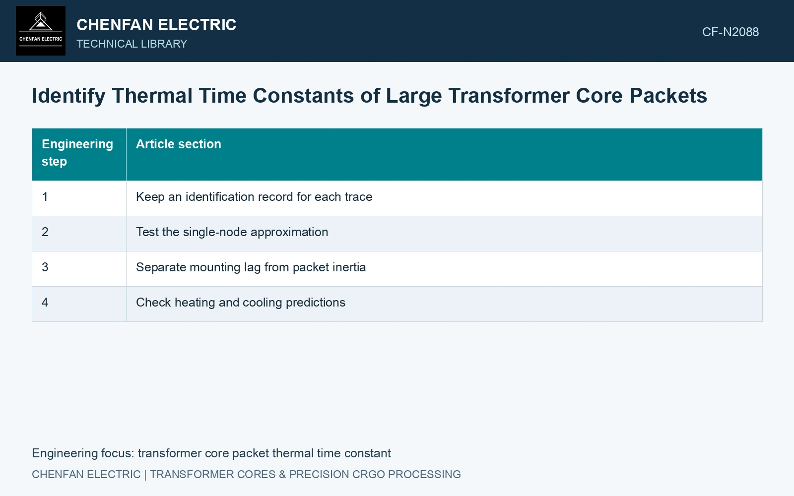
Keep an identification record for each trace
- Excitation
- Record the voltage, frequency, waveform and timing of changes that affect core heat generation.
- Cooling boundary
- Record adjacent fluid or air temperatures, cooling state and relevant flow changes.
- Measurement location
- Identify packet coordinates, surface or embedded position and the material hosting the sensor.
- Sensor response
- Retain calibration, mounting and independent response information where available.
- Initial condition
- Record the pre-test thermal state rather than assuming every region starts at ambient.
Test the single-node approximation
For a first-order lumped model with constant heat input and a fixed boundary, the rise follows θ(t)=θ∞[1−exp(−t/τ)]. At t=τ it reaches approximately 63.2% of its final rise. In that model τ=C/G, where C is thermal capacitance and G the total linearized conductance to the boundary.
Those relations are a model test, not a universal core law. If the interior and surface differ materially, the packet may require several nodes or a distributed description. Temperature-dependent loss and changing natural convection can also make the response depart from one exponential.
Do not calculate the 63.2% time from an uncertain final rise and call it a measured constant. A test stopped before a defensible endpoint may leave the fitted gain and time constant strongly dependent on one another.
Separate mounting lag from packet inertia
A probe in a spacer or support records through its host material and attachment. Include that heat path and its measured response in the identification; a slow recorded trace may combine sensor lag with packet inertia. [2]
Compare sensors with different, documented thermal paths, and include their response in the identification where necessary. Deconvolution without a credible sensor model can amplify noise and create an artificial fast core response.
Check heating and cooling predictions
Fit a simple model first, then inspect residuals across time and location. Persistent fast and slow residual components suggest that one node is insufficient. Validate against another input change or a cooling trace with its boundary measured; refitting the same trace does not test prediction.
Take an assumed 100 kg packet represented by 23ZH90, whose catalogue limit is 0.90 W/kg at 1.7 T and 50 Hz. [3] Its strip-input screen is 90 W. For an assumed first-order fit with 18 K final rise and thermal capacitance 45,000 J/K, G = 90/18 = 5 W/K and τ = C/G = 9,000 s = 150 min. At 150 min the predicted rise is 18(1 − exp(−1)) = 11.38 K. If the test stops at 60 min, the prediction is only 5.93 K; treating that reading as the final rise would greatly overestimate conductance. Extend the observation or bound the fit before releasing a time constant.
Packet mass, duct layout, contact compression and support paths determine the fitted capacitance/conductance combination. A time constant from another sheet count or clamp configuration needs renewed validation.
Deliver the thermal model, parameter evidence and applicable duty range. Retain heating–cooling differences and identify sensor or fluid effects that remain unresolved.
References
- Z. Chen, Z. He and S. Wang, Transformer Iron Core Temperature Field Calculation Based on Finite Element Analysis, Energies 18, 6537, 2025. DOI: 10.3390/en18246537.
- U.S. Department of Energy, DOE-HDBK-1012/2-92, Thermodynamics, Heat Transfer, and Fluid Flow, Volume 2, 1992.
- Nippon Steel Corporation, Grain-Oriented Electrical Steel Sheets, catalogue D004je, April 2020, specification and typical-property tables.