

Winter low-load operation still heats an energized core while tank and cooler boundaries remove heat unevenly. Map local steel and oil temperatures to distinguish core heat removal from cold-weather stratification. [1] [2]
Map the temperature around the core in height and across the nearby return paths. The purpose is to identify stratification and weakly mixed regions, not to diagnose a hot spot from a single top-oil number.
Separate the sources and sinks
Record core excitation, winding load and cooling-system state. Use the actual loss inputs; scaling all internal heat with load current removes the core source incorrectly. Record ambient conditions and relevant tank-wall exposure as time histories when the weather is changing.
Use fluid properties over the cold-to-warm range in the construction. A constant warm-oil viscosity can misrepresent hydraulic resistance in a cold return region. Temperature-induced density differences drive natural circulation, while the connected paths and their resistance determine where it flows.
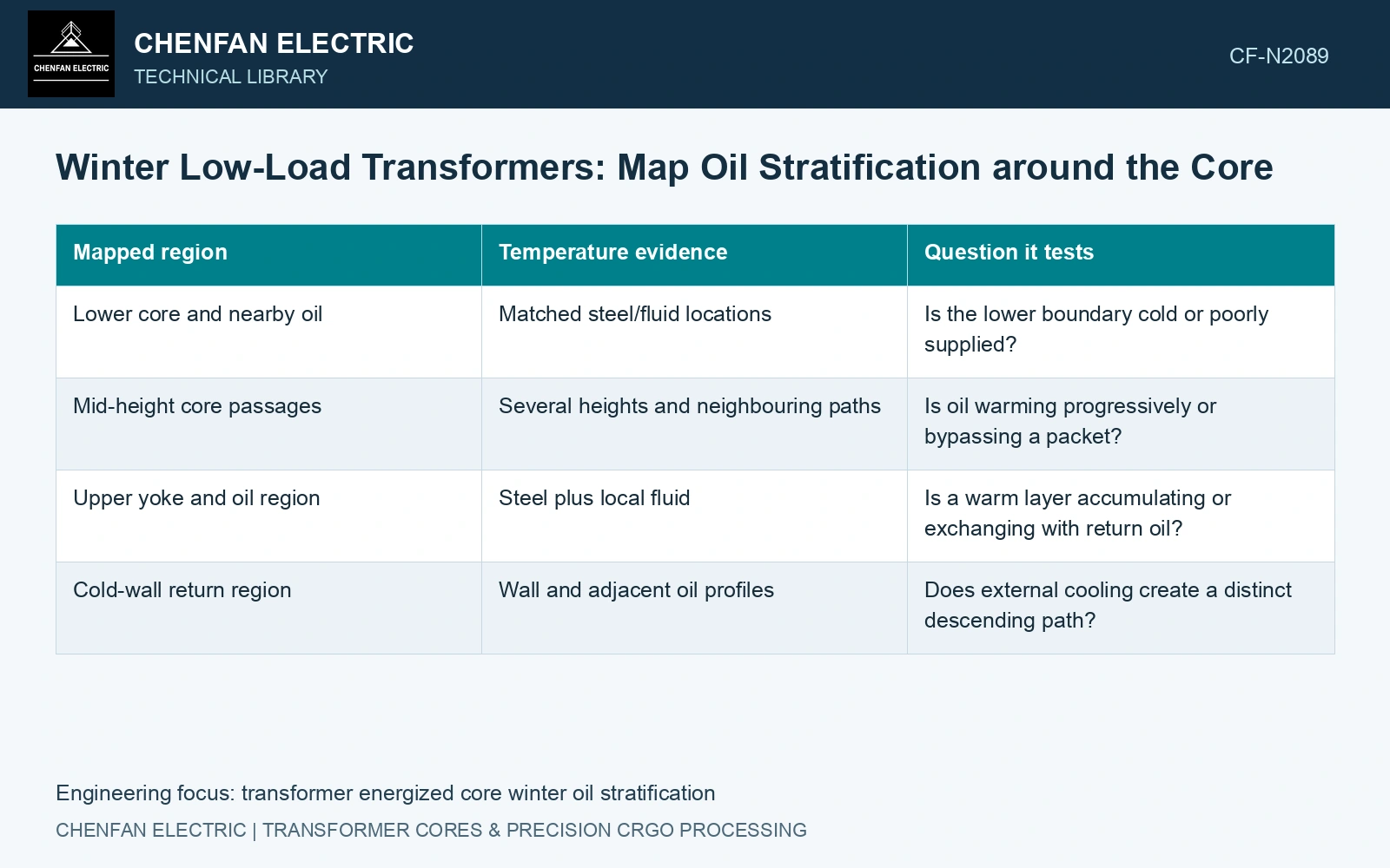
Build a vertical evidence map
| Mapped region | Temperature evidence | Question it tests |
|---|---|---|
| Lower core and nearby oil | Matched steel/fluid locations | Is the lower boundary cold or poorly supplied? |
| Mid-height core passages | Several heights and neighbouring paths | Is oil warming progressively or bypassing a packet? |
| Upper yoke and oil region | Steel plus local fluid | Is a warm layer accumulating or exchanging with return oil? |
| Cold-wall return region | Wall and adjacent oil profiles | Does external cooling create a distinct descending path? |
Attach elevations and horizontal positions to each reading. Measurements at the same height on opposite sides can test whether a one-dimensional stratification model is adequate. A vertical gradient alone does not establish the local velocity or prove stagnation.
Compare time-aligned steel and oil response
Observe how the map changes as ambient conditions, load or cooling state change within the permitted duty. Preserve enough initial-condition information to distinguish a cold-start transient from an established low-load state.
Check the predicted local flow direction where gradients or restrictions suggest weak circulation. Resolve the actual oil paths and compare local temperature and signed-flow evidence. A gradient alone does not establish a circulation threshold for this construction.
Use a 23ZH90 strip-input budget at its catalogue condition of 1.7 T, 50 Hz. [3] An assumed 1,000 kg region gives 900 W at 0.90 W/kg. If an assumed 600 W leaves through an upper oil branch carrying 0.040 kg/s with heat capacity 1,900 J/(kg·K), its bulk rise is 7.89 K; at 0.020 kg/s it is 15.79 K. The same source therefore permits very different vertical oil gradients. Instrument branch inlet and outlet temperatures and establish flow direction before interpreting an upper-core reading as evidence of increased magnetic loss. The 600 W split is an assumption to be checked, not a measured allocation.
Duct spacer positions, packet alignment and support footprints control the local passages. Preserve those dimensions and the oil fill state when comparing winter no-load records against warmer-duty baselines.
Compare steel-to-oil differences with regional boundary temperatures. Use those relationships to identify a restricted packet heat path or a circulation and mixing issue.
References
- Z. Chen, Z. He and S. Wang, Transformer Iron Core Temperature Field Calculation Based on Finite Element Analysis, Energies 18, 6537, 2025. DOI: 10.3390/en18246537.
- U.S. Department of Energy, DOE-HDBK-1012/2-92, Thermodynamics, Heat Transfer, and Fluid Flow, Volume 2, 1992.
- Nippon Steel Corporation, Grain-Oriented Electrical Steel Sheets, catalogue D004je, April 2020, specification and typical-property tables.