

An NGR purchase specification may guarantee resistance at a stated temperature. The fault does not remain at that temperature. As the elements heat, their resistance can change, and the current may depart from the value calculated using the cold measurement. [1]
Couple resistance to the electrical circuit
Within a justified limited temperature range, an illustrative linear model is R(T) = R0[1 + α(T − T0)]. R and R0 are in ohms; T and T0 are temperatures in degrees Celsius; α is the local resistance temperature coefficient in inverse kelvins. R0 applies at reference temperature T0. The expression is not a substitute for a verified curve outside its valid range.
If a fixed neutral voltage V in volts is applied across a purely resistive branch, I = V/R(T) and P = V²/R(T), with I in amperes and P in watts. For a positive α, current and power decrease as the resistance rises under this assumption. A real system can have changing neutral voltage and significant series impedance, so that conclusion must be checked in the complete network.
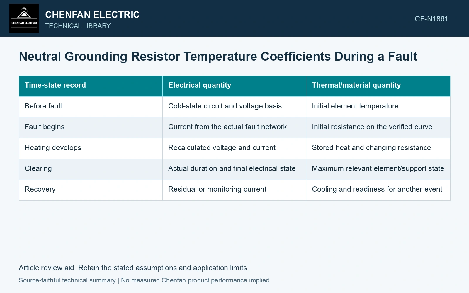
| Time-state record | Electrical quantity | Thermal/material quantity |
|---|---|---|
| Before fault | Cold-state circuit and voltage basis | Initial element temperature |
| Fault begins | Current from the actual fault network | Initial resistance on the verified curve |
| Heating develops | Recalculated voltage and current | Stored heat and changing resistance |
| Clearing | Actual duration and final electrical state | Maximum relevant element/support state |
| Recovery | Residual or monitoring current | Cooling and readiness for another event |
Keep the cold guarantee useful
A resistance tolerance at a reference temperature remains valuable manufacturing evidence. It establishes a reproducible comparison point. It does not certify hot current, thermal endurance or the behavior of a support exposed to uneven heating.
Ask for the material curve and duty assumptions behind the fault assessment. If only a single coefficient is supplied, identify the temperature range it represents. A linear extrapolation that produces a convenient current reduction can overstate the apparent thermal margin.
For the fixed-voltage resistive screen, calculate current and dissipated power at each resistance state using the same RMS voltage boundary. [2] Then carry the state-dependent current into the actual detection and clearing model.
Couple an assumed material slope to current
Assumptions: R₀ = 100 Ω at 20 °C, local coefficient 0.0004 K⁻¹ valid through 220 °C, and constant branch voltage 1,000 V RMS. At 220 °C, R = 108 Ω, I = 9.259 A and P = 9.259 kW, versus 10 A and 10 kW cold. Suppose an illustrative detection function requires current to remain above 9.50 A and has no hysteresis. The current crosses that boundary at R = 1,000/9.50 = 105.263 Ω, or T = 151.58 °C on this assumed curve. A design checked only at the cold 10 A would miss the later loss of that condition. Verify the real pickup/dropout/timer logic against the temperature/current trajectory before accepting clearing; the coefficient and boundary are example inputs, not alloy or relay guarantees.
Revisit protection using the current trajectory
The hot-current trajectory can cross a protection boundary even when the cold resistance passed inspection. Check detection and clearing against the verified R(T) curve and the full fault network. A calculated reduction in V²/R does not by itself establish a lower peak temperature if clearing lasts longer.
References
- IEEE, IEEE C57.32-2015, IEEE Standard for Requirements, Terminology, and Test Procedures for Neutral Grounding Devices (historical edition).
- U.S. Department of Energy, DOE-HDBK-1011/3-92, Electrical Science, Volume 3, June 1992.