

Distributed temperature sensing can provide a useful route profile, but the measured temperature belongs to the sensing fiber. A fiber alongside the jacket, inside a duct or in another cable location does not directly measure the conductor’s hottest point. That temperature is an estimate with a model behind it. [1]
The reliability of the estimate depends on the entire chain from optical measurement to thermal decision. Each link should have an identifiable input and limitation.
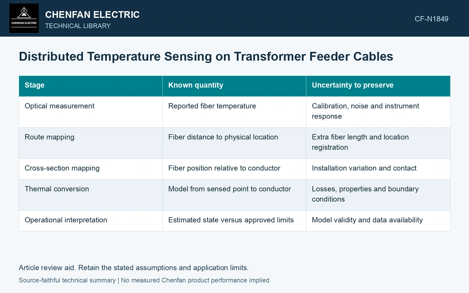
Follow the temperature through five stages
Start with the instrument’s reported fiber temperature and its calibration evidence. Map distance along the fiber to actual route positions, including joints, loops and changes of installation. Then identify the fiber’s position relative to the cable cross-section and external environment.
| Stage | Known quantity | Uncertainty to preserve |
|---|---|---|
| Optical measurement | Reported fiber temperature | Calibration, noise and instrument response |
| Route mapping | Fiber distance to physical location | Extra fiber length and location registration |
| Cross-section mapping | Fiber position relative to conductor | Installation variation and contact |
| Thermal conversion | Model from sensed point to conductor | Losses, properties and boundary conditions |
| Operational interpretation | Estimated state versus approved limits | Model validity and data availability |
A precise optical reading does not remove uncertainty in the fourth stage. If the cable loss, duct condition or fiber contact changes, the same fiber temperature can correspond to a different internal temperature.
Use electrical duty as part of the model
The model should receive the relevant current history and cable loss assumptions. Metallic-layer and dielectric losses can matter depending on construction and bonding. Treating all heat as conductor loss can distort the temperature difference between conductor and fiber.
External heat sources also need representation. A nearby hot pipe may warm the fiber and conductor differently. The model must distinguish that heat input from the feeder’s own losses, especially at a local crossing or duct entry.
Validate at the installation you will operate
Validation should compare predicted and credible measured quantities under defined loading and environmental conditions. A model that matches one low-load state may still have the wrong transient response at higher duty. Review heating and cooling behavior, not only a single fitted offset.
A temperature decision needs the uncertainty of the complete conversion model, not only the optical channel. Include calibration and thermal-model contributions and retain covariance where inputs share a cause. [2]
Check whether the conductor estimate has usable margin
Assumptions: the fiber measures 65 °C at a limiting location and a validated thermal conversion adds 20 K at the assessed load, giving an 85 °C conductor estimate. Independent standard uncertainties are 0.5 K for the optical reading and 4 K for the conversion, so uc = √(0.5² + 4²) = 4.03 K. With assumed coverage factor 2, the upper decision value is 85 + 8.06 = 93.06 °C. Against an assumed project conductor gate of 90 °C, a rule requiring the entire expanded interval below the gate is not met, despite a 5 K nominal margin. Hold an increase in feeder rating until uncertainty or loading is reduced. Separately verify that spatial filtering can resolve the limiting region. [1][2]
References
- J. Cho, J.-H. Kim, H.-J. Lee, J.-Y. Kim, I.-K. Song and J.-H. Choi, Development and Improvement of an Intelligent Cable Monitoring System for Underground Distribution Networks Using Distributed Temperature Sensing, Energies 7, 2014, sections 2–4.2.2. DOI: 10.3390/en7021076.
- B. N. Taylor and C. E. Kuyatt, NIST Technical Note 1297, Guidelines for Evaluating and Expressing the Uncertainty of NIST Measurement Results, 1994, sections 5 and 6.