

A feeder’s average route temperature is stable, yet one joint is becoming hotter. There is no contradiction. A small local region contributes little to a long spatial average, and the sensor may not be located on the thermal path closest to the joint’s internal heat source. [1]
The investigation should preserve three separate objects: the electrical joint, its heat-transfer path and the measurement system. Combining them into one cable-temperature value makes a localized fault difficult to interpret.
Start with the local source
Current through a resistive joint generates heat. A changed contact condition can raise local loss without a major change in total feeder current. The joint construction and its surroundings determine how that heat reaches the accessible surface or nearby sensing fiber.
A hot surface can also reflect an external source. Compare the suspected joint with nearby cable and environmental conditions before attributing the entire temperature difference to contact resistance. Thermal evidence can identify a location for qualified assessment; it does not uniquely establish the electrical mechanism.
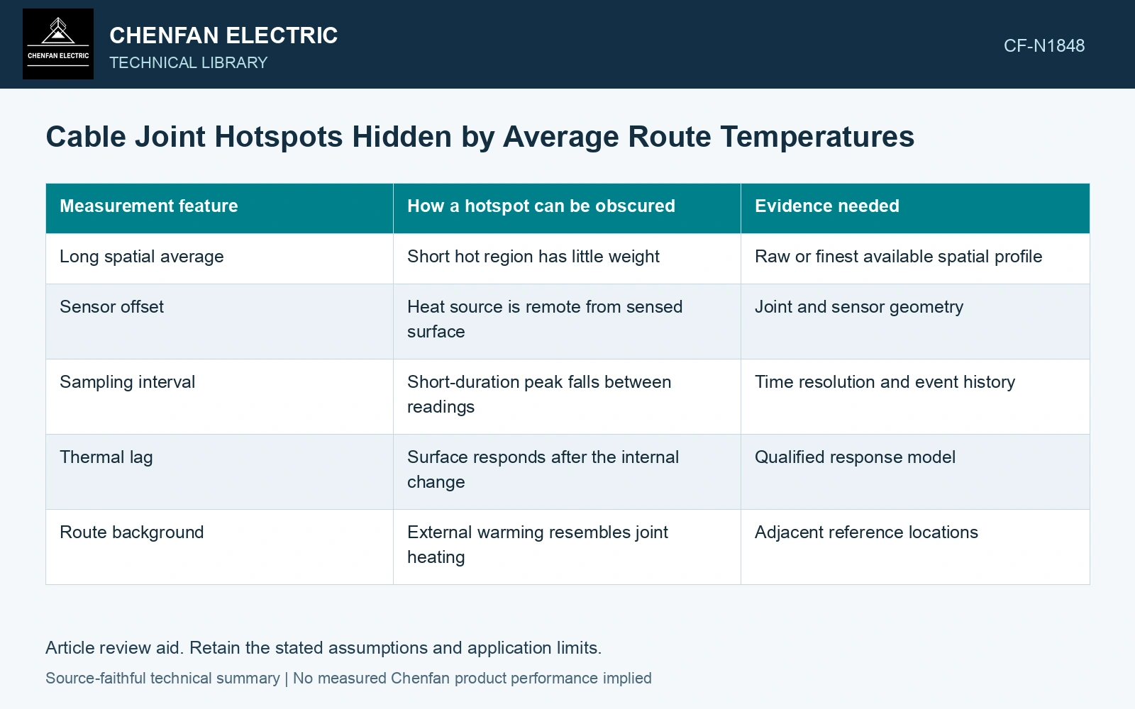
| Measurement feature | How a hotspot can be obscured | Evidence needed |
|---|---|---|
| Long spatial average | Short hot region has little weight | Raw or finest available spatial profile |
| Sensor offset | Heat source is remote from sensed surface | Joint and sensor geometry |
| Sampling interval | Short-duration peak falls between readings | Time resolution and event history |
| Thermal lag | Surface responds after the internal change | Qualified response model |
| Route background | External warming resembles joint heating | Adjacent reference locations |
Calculate what an average can conceal
For this assumption, suppose a 1 m region is 30 K above its surrounding 99 m section. A simple length-weighted average over 100 m rises by only 0.3 K. This arithmetic assumes an ideal average and uniform background. It says nothing about a real sensor’s spatial response or a joint’s permissible temperature.
The example explains why an innocuous average cannot rule out a local issue. The actual system’s spatial resolution, filtering and placement must be known before interpreting a flat profile.
Compare changes at matched duty
A joint-region trend should be examined alongside feeder current and ambient or route temperature. Higher current naturally changes heat input. Comparing two readings at different duty can exaggerate or conceal a developing difference. Retain the data rather than normalizing with an unverified universal factor.
If a thermal model estimates internal temperature, document its geometry and validation basis. A model calibrated on straight cable may not represent a joint’s multilayer construction and local contact source.
Cho and co-authors place a sensing fiber around the joint kit and distinguish measured fiber/sheath temperature from a modeled conductor temperature. Verify the joint-specific sensing geometry before reusing a straight-cable conversion. [1][2]
Reproduce the hidden joint rise
Extend the same explicit uniform-temperature-averaging assumptions: a 5 m window centered on the 1 m, 30 K hot region shows 6 K, versus 0.3 K over 100 m. With an assumed alarm trigger of a 5 K increase, the short window triggers and the route average misses the event. Choose a joint-region channel/processing configuration that demonstrates detection of this target in a qualification test. These ideal post-processing averages are not a Raman instrument response model; verify its actual point-spread function, fiber contact and internal-to-surface thermal lag. [1]
References
- J. Cho, J.-H. Kim, H.-J. Lee, J.-Y. Kim, I.-K. Song and J.-H. Choi, Development and Improvement of an Intelligent Cable Monitoring System for Underground Distribution Networks Using Distributed Temperature Sensing, Energies 7, 2014, sections 2–4.2.2. DOI: 10.3390/en7021076.
- U.S. Department of Energy, DOE-HDBK-1012/2-92, Thermodynamics, Heat Transfer, and Fluid Flow, Volume 2, 1992.