

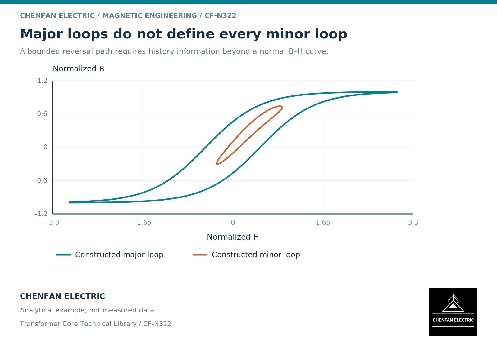
A major hysteresis loop and a minor loop answer different questions. A major loop describes a sufficiently large excursion under specified conditions; a minor loop records a smaller reversal within the magnetic history. A transformer study involving ripple, partial excursions or remanence may need the latter behavior even when a major-loop curve is available.
A reversal creates a path, not another point on one curve
A single-valued B-H relationship assigns one flux density B to each field strength H. Hysteresis instead permits different B values at the same H depending on the previous trajectory. Reversing excitation before completing a large excursion can create a nested path.
Basic magnetics guidance illustrates major and minor behavior, while constitutive-model documentation distinguishes reversible curves from history-dependent formulations. [1] [2] The important design question is which trajectories the intended duty actually visits.
A curve that reproduces the outer envelope may still misrepresent the slope and enclosed area of a smaller loop. That can affect a calculated current waveform or loss estimate without producing an obvious error in the plotted major loop.
Match the laboratory data to the intended trajectory
Request the excitation waveform, frequency, temperature, specimen orientation and conditioning associated with the data. For minor-loop use, identify the reversal levels and any bias around which the excursion occurs.
A set of isolated B-H points does not necessarily preserve the order in which the material traversed them. The data file should retain time or sequence information when fitting a history-dependent model. Otherwise the fitting process may interpret a loop as a noisy single-valued curve.
The specimen boundary also matters. A material coupon can support a constitutive model without reproducing all joints, stresses and multidirectional fields of an assembled core. Keep that distinction when translating laboratory parameters into a transformer model.
Separate stored energy from dissipated energy
For a closed magnetic cycle, the integral of H dB represents energy dissipated per unit volume under the applicable conditions. Multiplying a suitable cycle energy by the repetition rate gives an average power density. The units and cycle definition must remain explicit.
A smaller flux excursion does not justify scaling a major-loop loss simply by the ratio of peak densities. The path shape, reversal history and rate-dependent contributions can differ. If a loss model is used instead of an explicit hysteresis loop, state its calibration range and the waveforms it supports.
An illustrative diagram should show direction arrows and the nested reversal path. It should not label an invented loop as measured steel performance, and it should not use a visually convenient ellipse as a product’s actual characteristic.
Validate the behavior needed by the study
| Intended prediction | Useful validation evidence |
|---|---|
| Large excitation excursion | Outer-loop and high-field response |
| Ripple around a bias | Minor loops at relevant bias and amplitude |
| Remanence after interruption | History-dependent state evolution |
| Local rotating field | Directional or vector magnetic evidence |
Hold back at least one relevant trajectory from parameter fitting and use it as a separate check. A model that only reproduces the data used to tune it has demonstrated calibration, not independent predictive performance.
For procurement, the deliverable is not merely “a B-H curve.” It is a traceable dataset and a statement of which magnetic histories it can support. That information lets the transformer designer choose a model with enough memory for the actual duty, without assuming that the most elaborate model is automatically the best identified one.
References
[1] Lloyd Dixon / Texas Instruments. Magnetics Design 1 – Introduction and Basic Magnetics.
[2] Cesare Tozzo / COMSOL. Modeling Ferromagnetic Materials in COMSOL Multiphysics.