

A recorded PD waveform contains several pulses. They may represent separate sources, or one source followed by reflections at joints and cable ends. Counting every pulse as another defect can turn a useful measurement into a misleading location map. [1]
Begin with the circuit geometry and the measurement reference. The transformer-side termination may be a strong boundary in the tested arrangement, but its reflection behavior should come from the actual configuration. A termination label alone does not identify the signal path.
Label pulses before labeling defects
For each candidate event, preserve arrival time, polarity, waveform shape and amplitude within the measurement bandwidth. Compare repeated events for consistent timing. A similar delayed waveform can support a reflection interpretation, although dispersion and attenuation may change its appearance.
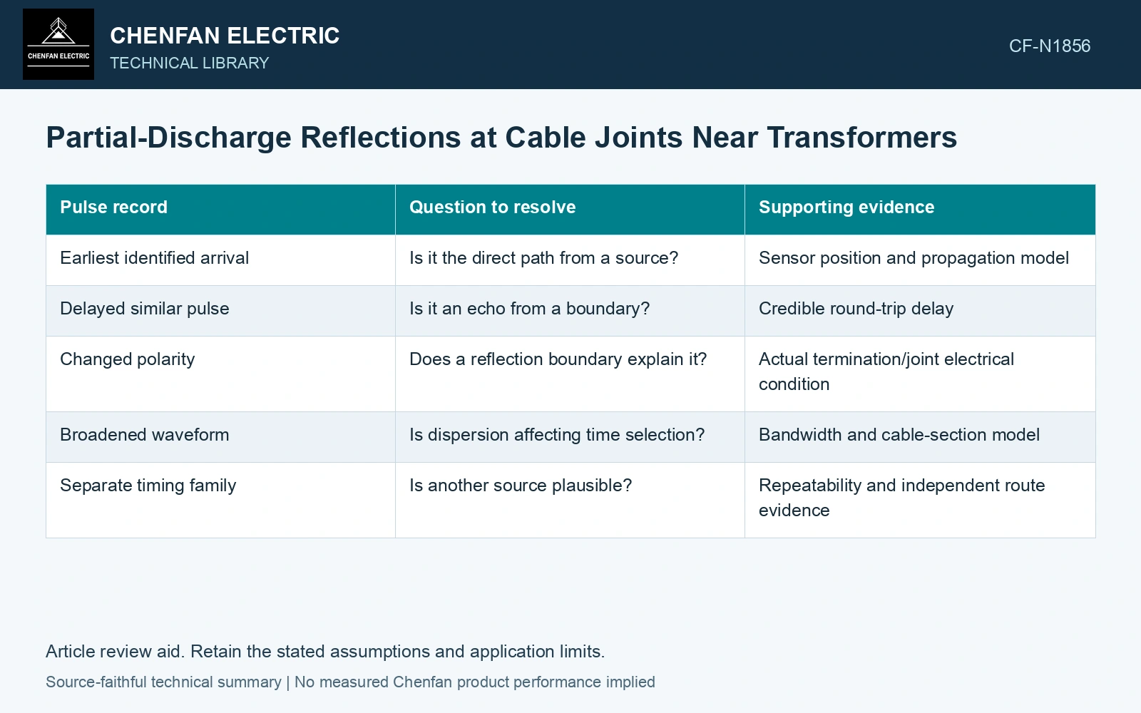
| Pulse record | Question to resolve | Supporting evidence |
|---|---|---|
| Earliest identified arrival | Is it the direct path from a source? | Sensor position and propagation model |
| Delayed similar pulse | Is it an echo from a boundary? | Credible round-trip delay |
| Changed polarity | Does a reflection boundary explain it? | Actual termination/joint electrical condition |
| Broadened waveform | Is dispersion affecting time selection? | Bandwidth and cable-section model |
| Separate timing family | Is another source plausible? | Repeatability and independent route evidence |
State the distance equation’s path
For a calibration pulse injected at the measurement end of a uniform cable, a confirmed round-trip reflection from a point at distance d gives d = vΔt/2. A PD source is a different geometry: if its direct pulse and far-end-reflected pulse are detected at the near end of a cable of length L, the source coordinate is x = L − vΔt/2. Label L, the sensor end and the selected pulse pair before converting time to position. [1]
If the path crosses different cable sections, travel time is the sum of each section length divided by its propagation speed. Replacing this with one unverified speed can shift an apparent location. The same issue arises when extra lead or test-system paths are included in the timing reference.
Use joint locations as evidence, not targets
Compare the estimated location and uncertainty with the route map. Include surveyed joint positions, mixed-section boundaries and route lengths. If two components fall inside the uncertainty range, retain both possibilities until evidence separates them.
Propagate the location model’s input uncertainties rather than attaching instrument timing accuracy to the final distance alone. Combined standard uncertainty must also include cable length, propagation speed and their covariance when relevant. [2]
Verify the reflection path before distance
Assumptions: a uniform cable is L = 500 m long, v = 160 m/μs, and the delay from the direct PD pulse to its identified far-end echo is 3 μs. Then x = 500 − 160×3/2 = 260 m from the sensor. The 240 m quantity is the distance from the source to the far end, not its sensor-end location. Assuming independent standard uncertainties uL = 1 m, uv = 2 m/μs and uΔt = 0.02 μs gives ux = √[1² + (3×2/2)² + (160×0.02/2)²] = 3.54 m. An assumed coverage factor of 2 gives 260 ± 7.09 m. A surveyed joint at 258 m is a candidate for follow-up; the 500 m termination is outside this interval. Do not count the echo as a second defect. [1][2]
References
- M. Shafiq, I. Kiitam, P. Taklaja, L. Kütt, K. Kauhaniemi and I. Palu, Identification and Location of PD Defects in Medium Voltage Underground Power Cables Using High Frequency Current Transformer, IEEE Access 7, 2019. DOI: 10.1109/ACCESS.2019.2930704.
- B. N. Taylor and C. E. Kuyatt, NIST Technical Note 1297, Guidelines for Evaluating and Expressing the Uncertainty of NIST Measurement Results, 1994, sections 5 and 6.