

A useful core optimum occupies a manufacturable region around its nominal geometry. Evaluate packet-build and joint variation to set production targets inside a demonstrated feasible range.
Inspect variations at the scale of the actual process. Infinitesimal slopes alone can miss a narrow optimum because the first derivative may be zero at its centre while curvature is large. [1]
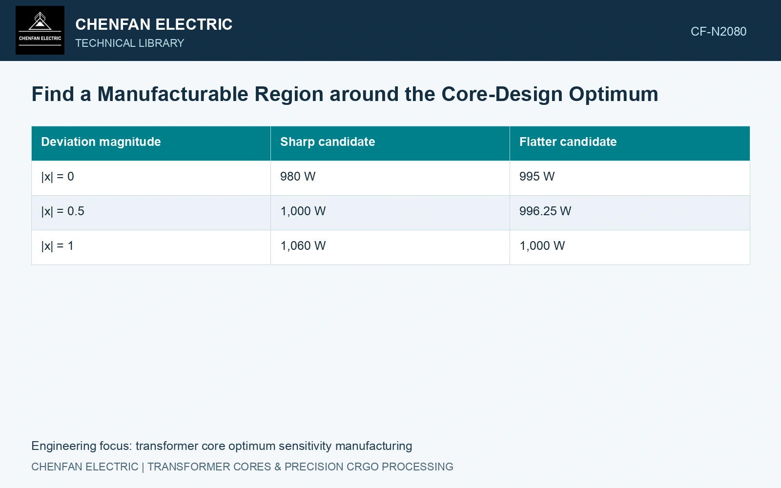
Compare manufacturable regions around each candidate
Consider two fictional loss responses. Let x denote a normalized manufacturing deviation, where |x|=1 is the assumed process range. Define Psharp=980+80x² W and Pflat=995+5x² W, with an illustrative limit of 1,000 W. These are explanatory equations, not measured core models.
| Deviation magnitude | Sharp candidate | Flatter candidate |
|---|---|---|
| |x| = 0 | 980 W | 995 W |
| |x| = 0.5 | 1,000 W | 996.25 W |
| |x| = 1 | 1,060 W | 1,000 W |
Both curves have zero slope at x=0. The sharp candidate has the better nominal loss but remains within the limit only for |x|≤0.5. The flatter candidate covers the full declared range. A centre-point gradient would not reveal that distinction.
Perturb the inputs that production actually varies
Use relevant packet dimensions, joint gaps, assembly pressure and coherent material properties. Preserve their physical relationships. If packet thickness and effective area move together, perturbing one while freezing the other can produce an artificial sensitivity.
Explore joint variations where interactions are credible. A design may tolerate a gap change and a pressure change separately yet fail when both occur together. Include permitted discrete transitions such as an extra layer or different spacer, which a local smooth response cannot represent.
Keep numerical instability separate from manufacturing sensitivity. Repeat mesh and solver checks where the response changes abruptly. An irregular loss surface caused by remeshing should not be interpreted as a factory’s process window.
Map the feasible production region
For each candidate, show the input region passing all requirements, not just the loss cap. Temperature, excitation, dimensions or noise may create a different limiting boundary. Overlay the credible process range or distribution with uncertainty in that range made visible.
If a probability model is justified, estimate the joint pass probability. If the requirement is to cover every permitted input bound, compare bounded regions instead. Those objectives lead to different statements and should not be exchanged merely to improve the headline result.
Use the catalogue nominal gauge of 0.23 mm to connect the normalised process coordinate to a real stack. [2] Assume 1,000 laminations, a nominal uncoated thickness sum of 230 mm, and a qualified total-thickness deviation of ±2 mm defining x = ±1. The sharp candidate’s acceptable |x| ≤ 0.5 then permits only ±1 mm around that nominal stack; the flatter candidate covers ±2 mm. These are assumed design responses and process bounds, not catalogue gauge tolerances. Select the flatter candidate if production cannot demonstrate the narrower band; a 15 W nominal advantage is insufficient when its feasible manufacturing interval is half as wide.
Sheet-count verification, measured gauge distribution, coating build and controlled compression establish the process coordinate. Determine its distribution from the actual stacking process instead of reading it from nominal strip thickness.
Confirm the stable region on representative constructions. Place drawing and process targets inside that region with achievable tolerances, pricing any nominal performance tradeoff against reduced sorting and correction.
References
- NIST/SEMATECH, e-Handbook of Statistical Methods, Response surface designs, section 5.3.3.6.
- Nippon Steel Corporation, Grain-Oriented Electrical Steel Sheets, catalogue D004je, April 2020, specification and typical-property tables.