

Joint temperature patterns reflect local magnetic loss and heat spreading through laminations, interfaces and supports. Model both to identify the construction change that can lower the governing temperature. [1] [2]
Keep the joint’s loss distribution as an input to this analysis. Recalculating its magnetic mechanism is a separate task; replacing the distribution with one average watt density removes the local question before the thermal calculation begins.
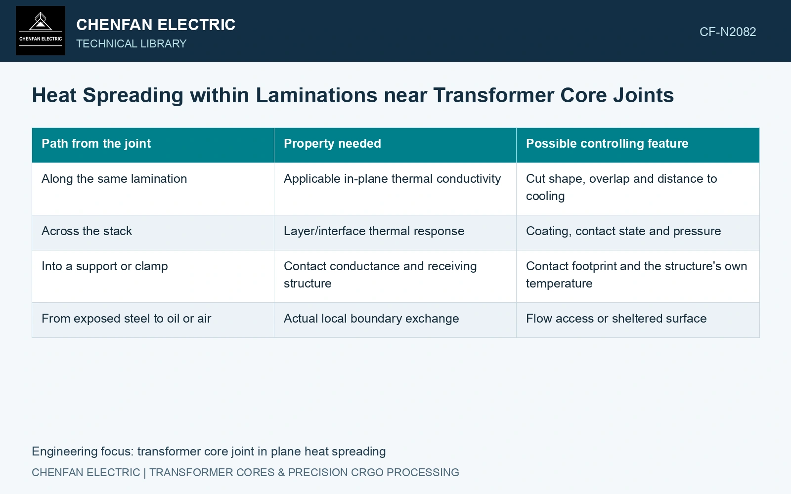
Follow the heat through the layer geometry
| Path from the joint | Property needed | Possible controlling feature |
|---|---|---|
| Along the same lamination | Applicable in-plane thermal conductivity | Cut shape, overlap and distance to cooling |
| Across the stack | Layer/interface thermal response | Coating, contact state and pressure |
| Into a support or clamp | Contact conductance and receiving structure | Contact footprint and the structure’s own temperature |
| From exposed steel to oil or air | Actual local boundary exchange | Flow access or sheltered surface |
Align the conductivity tensor with the physical layer axes. Thermal conductivity should come from thermal evidence; the rolling direction’s magnetic advantage does not establish an equivalent thermal-conductivity ratio. A scalar steel value applied to the whole coated packet can suppress the interface resistance that controls cross-stack spreading.
Use diffusion length with a defined purpose
For a simple directional transient screen, spreading length is of order √(αt), with diffusivity α in m²/s and elapsed time t in seconds. Use it to choose a resolution scale; it is not a hot-spot radius, steady influence distance or temperature prediction.
This is a scale for choosing spatial resolution or sensor spacing. It is not a hot-spot radius, a temperature prediction or a steady-state influence distance. Boundaries, source duration and other directions alter the actual field. A different through-stack diffusivity would give a different scale.
Compare the source footprint with the cooling path
Map the heated joint region, nearby overlaps, packet ends and wetted surfaces. Check whether a proposed sensor lies on the source, downstream of an effective spreading path or on a thermally separated lamination. Two equally distant points can respond differently because they do not share the same path.
Compare early and late temperature fields after a controlled excitation change. Early local response can help distinguish the source footprint from later heat spreading, but sensor mounting and response time must be included.
The 0.23 mm catalogue gauge gives a cross-layer length scale. [3] With an assumed in-plane diffusivity of 10⁻⁵ m²/s, the existing 100 s screen gives √(10⁻⁵ × 100) = 31.62 mm; by comparison, the notional diffusion time across one sheet is (0.00023)²/10⁻⁵ = 0.00529 s. Applying that sheet value through a 23 mm packet would predict 52.9 s, but only if interlaminar contacts had no additional resistance. They do. Retain directional effective properties and measured contact effects for the packet; do not use a single-sheet calculation to dismiss a joint-localised temperature gradient.
Joint overlap, sheet registration, coating integrity and compression define the cross-layer heat path. Resolve them separately from the comparatively rapid in-plane spreading inside an individual lamination.
Map heat generation and transport separately against measured temperatures. Revisit cross-stack interfaces when the packet appears too uniform and use the combined evidence to target the effective construction change.
References
- Z. Chen, Z. He and S. Wang, Transformer Iron Core Temperature Field Calculation Based on Finite Element Analysis, Energies 18, 6537, 2025. DOI: 10.3390/en18246537.
- U.S. Department of Energy, DOE-HDBK-1012/2-92, Thermodynamics, Heat Transfer, and Fluid Flow, Volume 2, 1992.
- Nippon Steel Corporation, Grain-Oriented Electrical Steel Sheets, catalogue D004je, April 2020, specification and typical-property tables.