

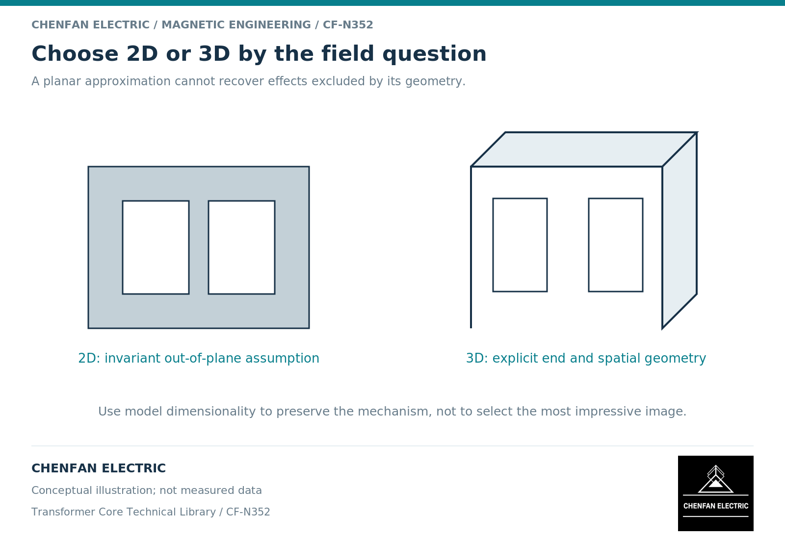
Choose two-dimensional or three-dimensional finite-element analysis from the field behavior that controls the decision. Three dimensions are necessary when the omitted direction contains important geometry or flux paths; they are not automatically a guarantee of accuracy. A well-validated two-dimensional model can be more useful than an under-resolved three-dimensional one.
Understand what the dimensional reduction assumes
A planar two-dimensional model usually represents a geometry and field behavior that are invariant in the omitted direction, with a defined depth for integrated quantities. An axisymmetric model represents rotation about an axis. These are different assumptions, not interchangeable ways to save computing time.
Finite-element documentation distinguishes planar and axisymmetric formulations and their output scaling. [1] A three-limb core is not axisymmetric merely because one winding is approximately circular.
Before reducing the model, identify the field components and geometric features that the reduction removes. End regions, leads, return structures and local openings may be central to one question and secondary to another.
Match the model to the observable
A section model may adequately compare limb-average flux or a local cross-sectional trend under a stated excitation. It may not reproduce a three-dimensional return through a tank, end-clamp losses or the field around a lead penetration.
Material direction also matters. A reduced model can represent anisotropy only within the assumptions and directions retained. A vector hysteresis benchmark illustrates how rotating fields and directional material response create demands beyond a simple scalar curve. [2]
| Question | Dimensional issue to examine |
|---|---|
| Average limb excitation | Validity of uniform depth and branch representation |
| Joint or opening field | Out-of-plane redistribution and local material axes |
| Winding-end leakage | Axial end geometry and return current paths |
| Tank or clamp loss | Three-dimensional conducting loops and field penetration |
| Comparative screening | Whether omitted effects cancel between candidates |
The last row is important: a reduced model may rank two similar options reliably even when it does not predict their absolute losses precisely. That use still requires evidence that the omitted effects do not change the ranking.
Use a hierarchy rather than one oversized model
Begin with analytical or magnetic-network checks, then a reduced field model where appropriate. Use targeted three-dimensional regions or a full model for the effects that control the conclusion.
Compare overlapping observables between levels. If a three-dimensional model predicts a very different total flux from a simple continuity calculation, investigate the discrepancy rather than assuming the more elaborate result is correct.
Keep excitation, material data and geometry definitions aligned across models. Otherwise the comparison changes several variables at once and cannot isolate the effect of dimensionality.
Report the omitted physics explicitly
The handover should state dimensionality, depth or axis definition, symmetry assumptions, represented structures and excluded regions. Include mesh and domain sensitivity, parameter sources and relevant validation cases.
A three-dimensional model still needs correct boundary conditions, material axes, current definitions and temporal treatment. It can fail through a wrong source or unsupported material curve just as a two-dimensional model can.
The useful engineering statement is that the selected dimensionality resolves the effects needed for a specified observable. Avoid saying simply that a design was “verified by 3D FEA.” Finite-element analysis is a method; the evidence lies in the model definition, convergence checks and comparison with independent physical information.
References
[1] David Meeker. Finite Element Method Magnetics User Manual.
[2] COMSOL. Vector Hysteresis Modeling.