

Short answer
Feeder-head transformer estimates should reconcile: power measured at the feeder head for an interval equals the sum of transformer-level loads for the same interval plus line and transformer losses. When they do not, the residual is evidence of mapping errors, missing loads, clock offsets or wrong loss estimates. In an illustrative peak hour, the head measures 10.0 MW, transformer estimates sum to 9.2 MW and calculated losses are 0.3 MW, leaving 0.5 MW. When sensor data split the feeder into sections, 0.4 MW of the residual sits in section 3, pointing to transformers there that are missing from the customer mapping. Reconciliation requires matching intervals, time stamps and loss calculations first. Calibration should then correct identified causes. Scaling every transformer estimate by the same factor to force a match hides the errors and distorts individual transformer loadings.
The balance
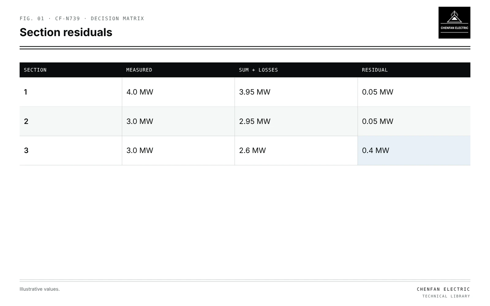
| Section | Measured | Sum + losses | Residual |
|---|---|---|---|
| 1 | 4.0 MW | 3.95 MW | 0.05 MW |
| 2 | 3.0 MW | 2.95 MW | 0.05 MW |
| 3 | 3.0 MW | 2.6 MW | 0.4 MW |
Phead = Σ Ptransformers + Plosses + Presidual
All terms for the same interval, at the same time base.
Alignment before comparison
- Interval length identical; 15-minute AMI against 1-minute SCADA needs aggregation.
- Time stamps: interval start versus end conventions; clock drift.
- Losses calculated for the same interval and load level; see technical and nontechnical losses at a distribution transformer.
- Unmetered loads added as estimates with flags.
Localising residuals
Illustrative example. Feeder with three sections bounded by line sensors. Peak hour: head 10.0 MW, transformer sum 9.2 MW, losses 0.3 MW. Values chosen for demonstration.
| Section | Measured | Sum + losses | Residual |
|---|---|---|---|
| 1 | 4.0 MW | 3.95 MW | 0.05 MW |
| 2 | 3.0 MW | 2.95 MW | 0.05 MW |
| 3 | 3.0 MW | 2.6 MW | 0.4 MW |
| Total | 10.0 MW | 9.5 MW | 0.5 MW |
Section 3 holds most of the residual. Field checks there might find transformers not linked to customers, a feeder boundary error in GIS, or a large unmetered load.
Calibration versus forcing
| Approach | Effect |
|---|---|
| Correct mapping and add unmetered loads | Residual falls for the right reason |
| Adjust loss model with measured data | Better loss estimates |
| Scale all transformers by head/sum | Matches total, hides local errors |
| Leave residual visible | Honest uncertainty |
Forced scaling makes transformers in correctly mapped sections appear more loaded than they are, and those in section 3 still under-represented.
Time behaviour
Residuals that vary with time of day suggest load types (for example street lighting at night); constant residuals suggest a missing large load or a clock shift. Comparing residuals across seasons separates heating or cooling loads.
Related methods: calibrating transformer load allocation with AMI data; hidden parallel paths that distort balances in normally open points without hidden parallel sources.
What this article does not cover
Nontechnical loss assessment at a single transformer is not repeated here.
Where this reasoning stops. Section values are illustrative; sensor accuracy adds its own uncertainty.
Practical takeaway
Align intervals, time stamps and losses, localise residuals with section measurements, correct mapping and unmetered loads, and avoid uniform scaling that forces a match.