

Short answer
Monte Carlo load scenarios for transformer studies go wrong when variables are sampled independently. Load, solar output, heating, cooling and EV charging all depend on weather, season and time of day. Drawing each from its own distribution produces combinations that never happen, such as full midday solar output with peak night-time heating and evening EV charging at the same instant. In an illustrative case, three variables with 10 bins each give 1,000 combinations, of which perhaps 40 % are physically impossible. These distort tail results, which are what transformer planning cares about. Sampling from joint historical profiles or weather-driven models keeps the correlations; operating rules such as tariff periods and control limits filter remaining invalid cases. Adequacy depends on whether the relevant regions are covered, not on how many runs were made. Simulation count is not the same as real sample size.
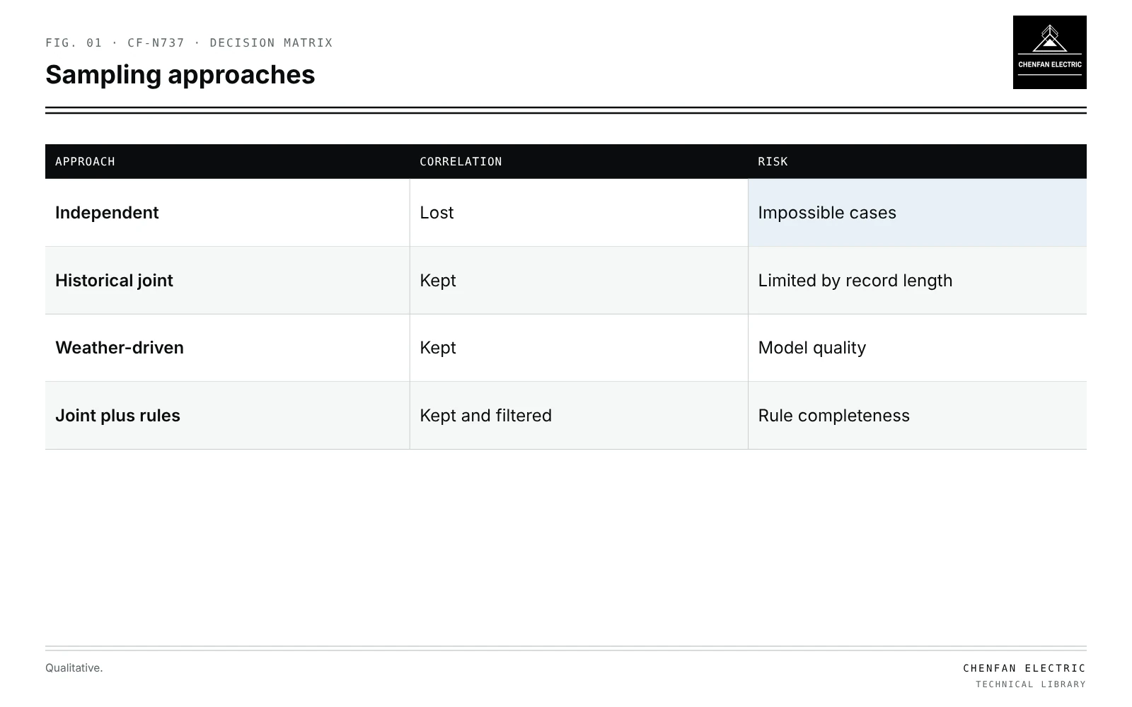
How independence fails
| Approach | Correlation | Risk |
|---|---|---|
| Independent | Lost | Impossible cases |
| Historical joint | Kept | Limited by record length |
| Weather-driven | Kept | Model quality |
| Joint plus rules | Kept and filtered | Rule completeness |
| Variable | Driven by |
|---|---|
| PV output | Irradiance, time of day, season |
| Heating load | Temperature, time of day |
| Cooling load | Temperature, irradiance |
| EV charging | Arrival time, tariff; see correlated EV charging loads |
| Base load | Day type, time |
Independent sampling breaks these links.
Counting impossible cases
Illustrative example. Three variables (PV, heating, EV) each binned into 10 levels. Values chosen for demonstration.
10 × 10 × 10 = 1,000 combinations
If maximum PV cannot occur at night and maximum heating cannot occur at summer midday, a large share of combinations, perhaps 40 %, is impossible. Worse, impossible combinations often sit in the tails, inflating or deflating extreme loading estimates.
Better sampling
- Historical joint profiles: sample whole days or weeks from records, keeping all variables together.
- Weather-driven models: sample weather, then compute each load from weather and time.
- Copulas or conditional distributions where data are limited.
- Scenario layers: adoption levels for PV, EV and heat pumps sampled separately, then applied to joint profiles.
Operating rules
- Tariff periods fix when managed EV charging occurs.
- Inverter limits cap PV export.
- Control rules for storage and heat pumps.
Scenarios violating these are removed or corrected.
Coverage, not count
| Check | Question |
|---|---|
| Tail coverage | Are extreme but possible conditions sampled? |
| Season and day type | Are all represented? |
| Joint extremes | Are realistic co-occurrences present? |
| Convergence | Do results stabilise for the statistic of interest? |
Ten thousand runs drawn from one year of data still represent one year of weather. The effective sample size is limited by the source data.
Results feed hosting capacity and capacity planning; see probabilistic hosting capacity and planning transformer capacity with electrification scenarios. Input sensitivity is covered in sensitivity ranking for planning inputs; time-series simulation in quasi-static time-series studies.
What this article does not cover
It does not treat the number of simulations as equivalent to real sample size.
Where this reasoning stops. The impossible share is illustrative; it depends on variables and climate.
Practical takeaway
Sample load scenarios jointly from weather and time, filter by operating rules, check coverage of tails and seasons, and report the data basis rather than the run count.