

An external sensor can receive gas, support and tank-wall paths. Wang et al.’s oil-array model explicitly omits tank-wall sound transmission [1]; that model cannot validate an external gas-transformer location estimate.
This matters when a location algorithm is borrowed from an oil-filled transformer. Even a well-calibrated oil sound-speed value describes the wrong medium. The gas identity, operating temperature, internal construction and tank-wall propagation need their own treatment.
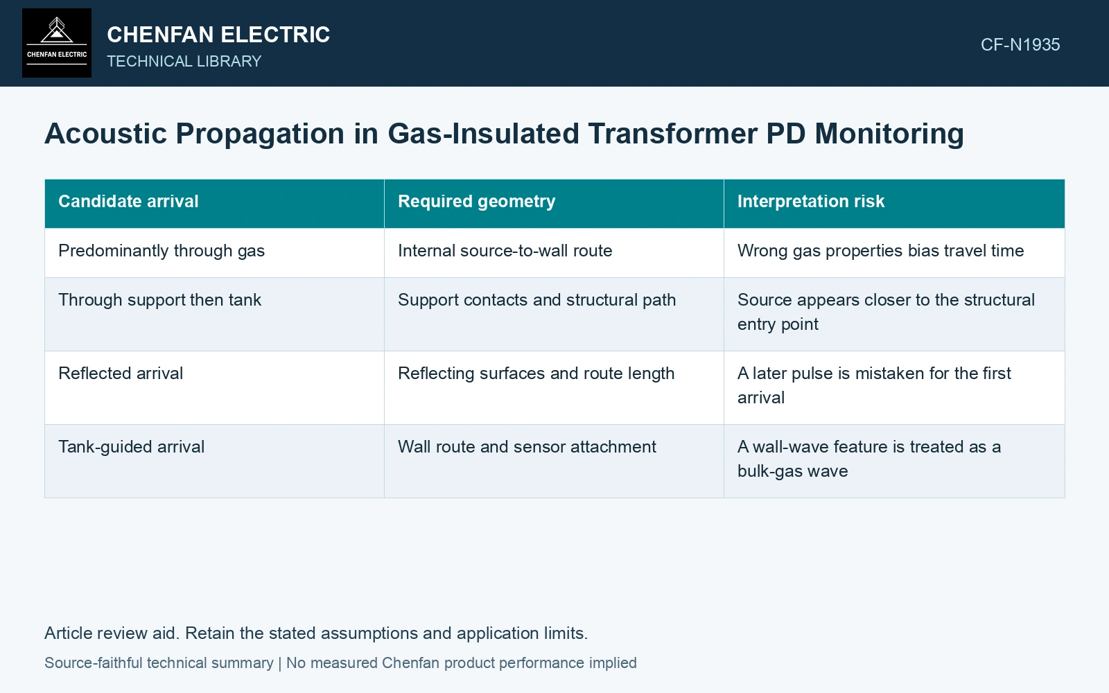
Build a path model before fitting a position
For a proposed path containing several segments, its travel time is t = Σ(Lj/cj). Segment length Lj is in metres, wave speed cj is in metres per second, and t is in seconds. This calculation assumes each segment’s speed is adequately represented and excludes additional sensor or processing delay unless those are added separately.
Compare plausible routes rather than selecting one speed for the entire distance. A short gas crossing followed by a long metal-wall route may compete with a longer direct gas crossing. Interfaces can also change amplitude, so the mathematically earliest route may be too weak to identify in the measured record.
| Candidate arrival | Required geometry | Interpretation risk |
|---|---|---|
| Predominantly through gas | Internal source-to-wall route | Wrong gas properties bias travel time |
| Through support then tank | Support contacts and structural path | Source appears closer to the structural entry point |
| Reflected arrival | Reflecting surfaces and route length | A later pulse is mistaken for the first arrival |
| Tank-guided arrival | Wall route and sensor attachment | A wall-wave feature is treated as a bulk-gas wave |
Separate property changes from sensor delay
Specify wave speed by gas composition and evaluated temperature/pressure, then identify the structural modes separately. Zhu et al. use couplant at a GIS shell-mounted sensor [2]; their study classifies selected defect models and does not validate source coordinates in a transformer.
Document the property model at the operating state. Keep sensor attachment, channel delay and detection thresholds in a separate uncertainty budget. Otherwise a change in adhesive coupling can be interpreted as a change in discharge location.
Use arrival differences carefully
If the acoustic source time is unknown, arrival-time differences remove that common unknown only when channels observe the same event and comparable path families. Subtracting a reflected arrival at one sensor from a direct arrival at another produces a precise number with the wrong geometric meaning.
Assume gas speed 150 m/s and steel-path speed 5,000 m/s at the evaluated state. A 1.0 m gas path takes 6.667 ms; a competing path of 0.05 m gas plus 0.95 m steel takes 0.523 ms. A borrowed oil-like 1,400 m/s model gives 0.714 ms for 1 m, matching neither route. These assumed paths show why the earliest detected signal may not follow the direct gas route. Retain path families, coupling and channel delays in calibration; one arrival cannot uniquely locate the discharge.
Controlled calibration observations can test whether the proposed geometry reproduces measured differences. They must also describe which propagation modes were excited; reproducing one accessible tank path does not validate every internal source position. Report a region and the competing path explanations when the observations cannot support a unique point. That is more useful for inspection planning than a coordinate whose apparent precision comes from an unsuitable sound-speed assumption.
References
- Y. Wang, D. Zhao, Y. Jia, S. Wang, Y. Du, H. Li and B. Zhang, Acoustic Sensors for Monitoring and Localizing Partial Discharge Signals in Oil-Immersed Transformers under Array Configuration, Sensors 24, 4704, 2024. DOI: 10.3390/s24144704.
- X. Zhu, C. Hu, J. Yang, Z. Liu, Z. Wang, Z. Liu and Y. Zang, Acoustic Identification Method of Partial Discharge in GIS Based on Improved MFCC and DBO-RF, Energies 18, 1619, 2025, section 2.1. DOI: 10.3390/en18071619.