

Peak flux under distorted voltage is determined by the maximum excursion of the induced-voltage integral, together with the initial magnetic state. Root-mean-square voltage alone does not provide that result. Two waveforms can have the same root-mean-square value and different peak flux trajectories.
Retain waveform shape and timing
For a winding with N turns, integrate e(t)/N to obtain the change in linked flux. [1] For each sinusoidal voltage component at frequency f_h, the corresponding ideal flux amplitude is proportional to its voltage amplitude divided by 2pi f_h N.
This frequency weighting is useful, but the total peak requires the components to be combined with their phase relationships. Summing their individual magnitudes gives a bound, not generally the actual maximum.
The initial flux adds another offset. A periodic centered reconstruction and a transient reconstruction starting from a residual state answer different questions. Label which one is being calculated.
An illustrative third-harmonic comparison
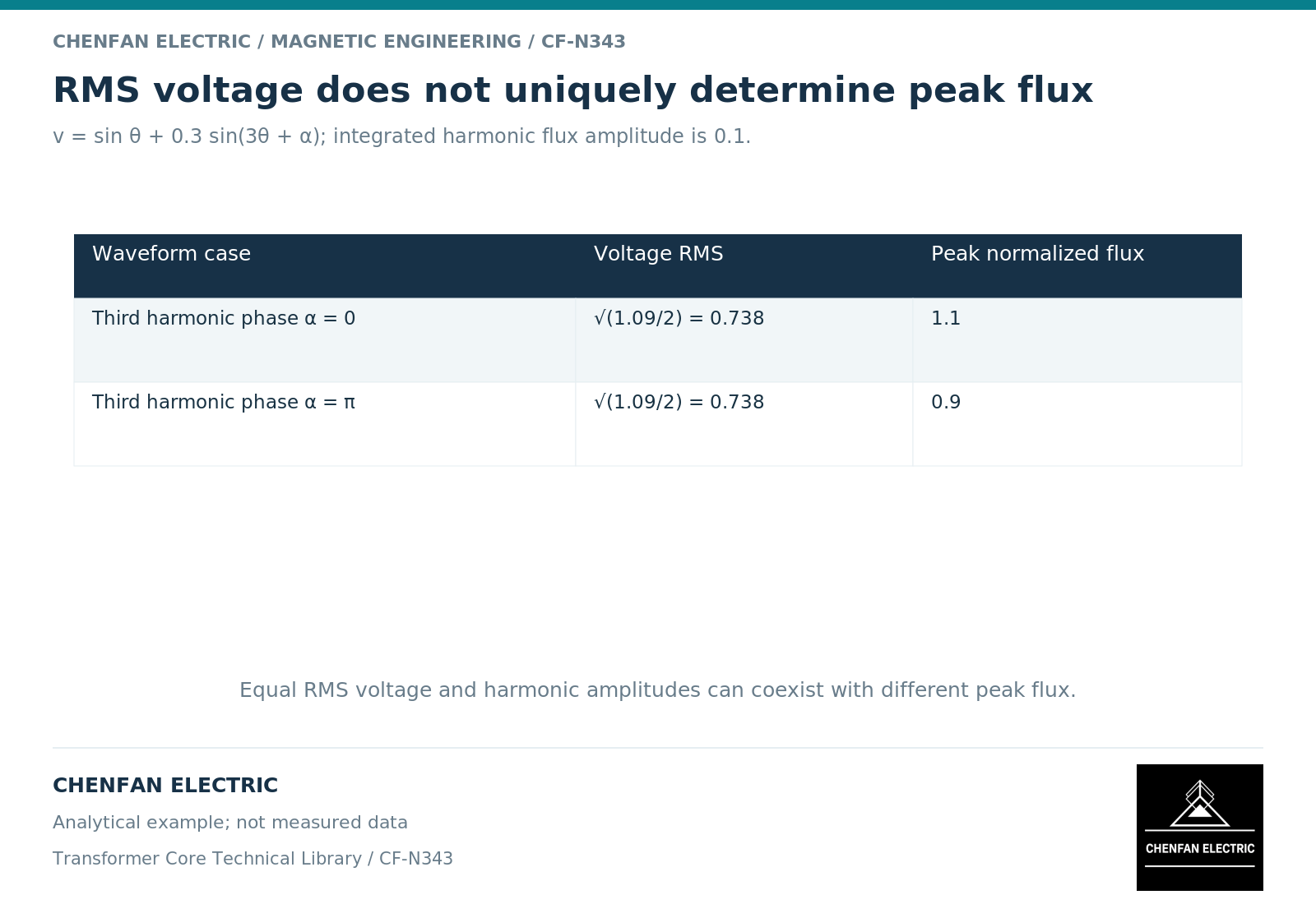
Take a normalized induced voltage v(x) = sin(x) + 0.3 sin(3x + theta), where x is the fundamental electrical angle. With an appropriate normalized flux scale, the centered flux is b(x) = -cos(x) – 0.1 cos(3x + theta).
For theta = 0, the maximum absolute value is 1.1. For theta = pi, the waveform becomes -cos(x) + 0.1 cos(3x), whose maximum absolute value is 0.9. Both voltage waveforms have the same component magnitudes and the same root-mean-square value, sqrt(1.09/2) in the chosen voltage scale.
These are analytical waveforms, not measured transformer records. They demonstrate that equal root-mean-square voltage and equal harmonic magnitudes do not establish equal peak flux. The phase relation changes the cumulative voltage-time area.
Check the terminal-to-induced-voltage approximation
At light excitation, the difference may be small enough for the intended screening. Under significant current, resistance and leakage-related drops can alter the induced voltage. A nonlinear transformer circuit should preserve the location of the magnetizing branch relative to those drops. [2]
A measured terminal waveform should therefore be accompanied by the assumptions used to reconstruct the core-driving voltage. Do not claim a direct measurement of local core density from terminal integration unless the required mapping and uncertainty have been established.
For three-phase cores, reconstruct the relevant phase winding quantities on a common time base. Line-to-line records may need a connection-specific interpretation; they do not reveal every common-mode component by themselves.
Report the flux result with its uncertainty
A useful output includes the original voltage waveform, the reconstructed induced voltage, the integrated trajectory and the positive and negative extrema. State turn count, tap position, net-area basis and the treatment of initial state and integration drift.
| Reported value | Supporting definition |
|---|---|
| Voltage root-mean-square | Measurement interval and channel reference |
| Harmonic amplitudes | Peak or root-mean-square, order and phase |
| Flux excursion | Integration interval and initial reference |
| Peak density | Net area and spatial averaging assumption |
| Uncertainty | Offset, scaling, timing and circuit approximation |
The result should be used to evaluate the magnetic operating envelope, not to infer core loss by a simple peak-density ratio. Loss also depends on the trajectory and material response. Keeping those two questions separate avoids replacing one incomplete scalar with another.
References
[1] Lloyd Dixon / Texas Instruments. Magnetics Design 1 – Introduction and Basic Magnetics.
[2] Manitoba Hydro International / PSCAD. The Classical Approach.