
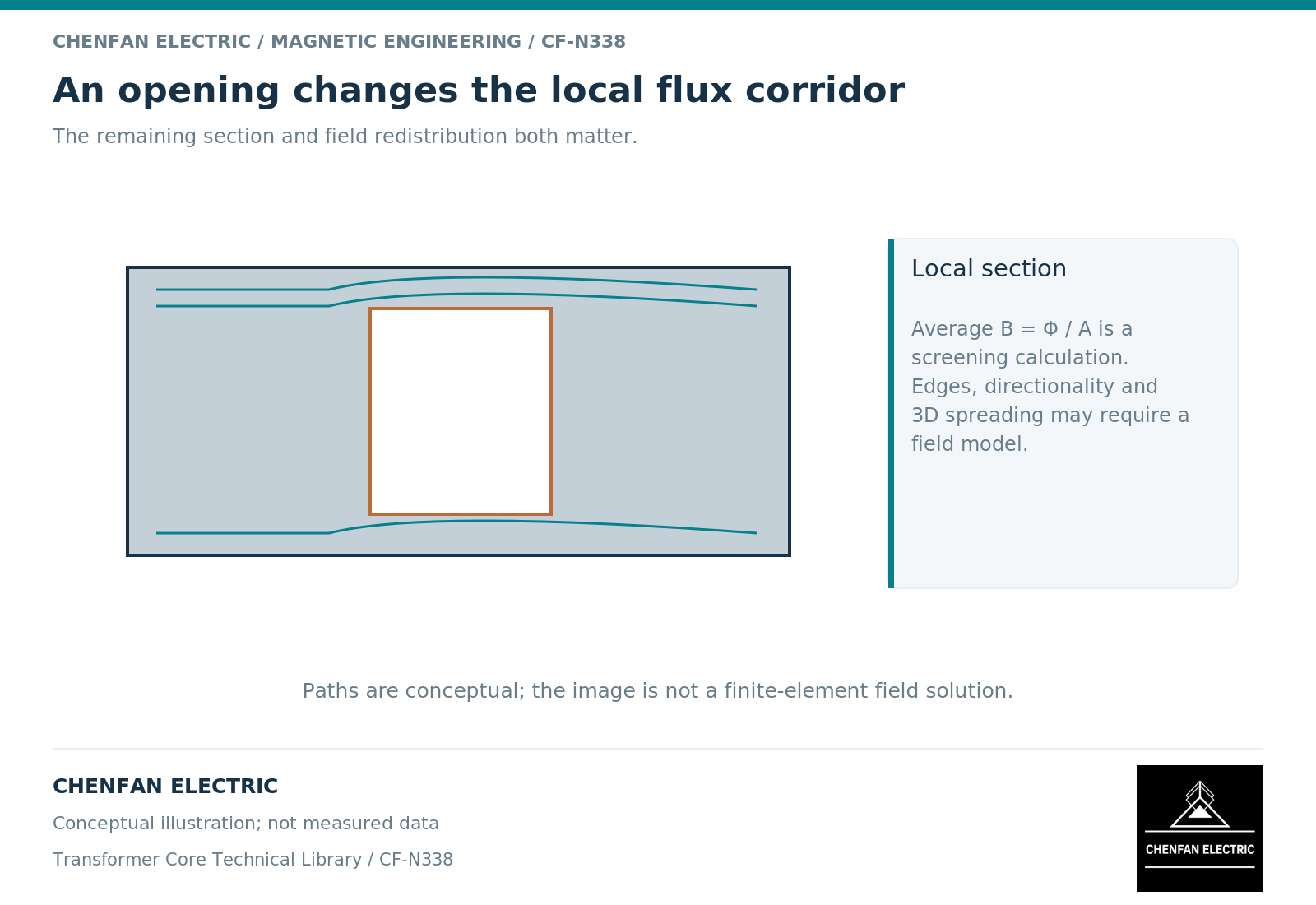
A structural opening can concentrate or redirect flux locally even when the average limb density remains acceptable. The relevant question is how the field passes around the opening and through the remaining magnetic section. A bulk area calculation is a useful screen, but it cannot describe every local direction change or hot spot.
Separate geometric diversion from manufacturing damage
This topic concerns the electromagnetic effect of the opening itself: removed magnetic area, altered path length and changed field direction. It is distinct from edge damage, burrs or mechanical stress introduced during manufacture.
Those effects may coexist in a real component, but combining them into one unexplained loss allowance makes diagnosis difficult. The model should state which are represented and which require separate material or manufacturing evidence.
A finite-element formulation can resolve spatial field variation subject to its geometry, material and boundary assumptions. [1] It should not be described as a measured result merely because the mesh follows a real drawing.
Use average-area arithmetic only as a first screen
Suppose an illustrative section carrying 0.010 weber has a net area of 0.008 square metre before an opening is introduced. Its average density is 1.25 tesla. If the effective remaining area at a restricted section is 0.007 square metre and the same flux crosses it, the average there becomes about 1.429 tesla.
This calculation does not predict the maximum density at the opening edge. Flux can redistribute through the three-dimensional region, and the field may turn relative to the steel’s preferred direction. The arithmetic simply identifies why the removed section deserves review.
Sharp idealized corners can also create mesh-sensitive peaks. A reported maximum at a mathematical corner should not be accepted without examining the actual radius and convergence behavior.
Preserve material direction and physical geometry
For grain-oriented steel, the local rolling direction must be mapped correctly. An isotropic model can miss the consequence of flux turning around an opening. Constitutive modeling distinguishes directional behavior from a scalar material relation. [2]
Use actual opening dimensions, edge radii, nearby joints and adjacent structural parts where they influence the question. Decide whether a two-dimensional section captures the dominant path or whether end effects require three dimensions.
The excitation should match the operating case. A balanced rated-voltage solution may not control a region under unbalance, bias or a transient. State which cases were screened and why.
Judge the result through multiple observables
| Check | Reason |
|---|---|
| Section-averaged flux density | Connects the field result to continuity |
| Local density and direction | Identifies concentration and off-axis excitation |
| Mesh refinement | Tests whether the reported peak is numerical |
| Integrated loss | Checks the overall energetic consequence |
| Local thermal assessment | Evaluates concentrated heat under the duty |
A single colored contour is insufficient. Request consistent scales for compared designs, the physical location of the reported maximum and the change in the engineering quantity that drives the decision.
For the manufacturing handover, freeze the evaluated opening geometry and its location relative to packet orientation. A change that looks minor on a mechanical drawing can alter the local magnetic path. The acceptance decision should come from the responsible design assessment, not from a generic claim that the average limb density remains unchanged.
References
[1] David Meeker. Finite Element Method Magnetics User Manual.
[2] Cesare Tozzo / COMSOL. Modeling Ferromagnetic Materials in COMSOL Multiphysics.