

An optimizer may label two GOES grades as 1 and 2. A value of 1.4 is a mathematical interpolation, not a purchasable material. Keep each real grade’s property and process set together rather than averaging labels.
Keep grade selection discrete. Use gradient information for suitable continuous variables within a specified grade branch, then compare the complete feasible branches.
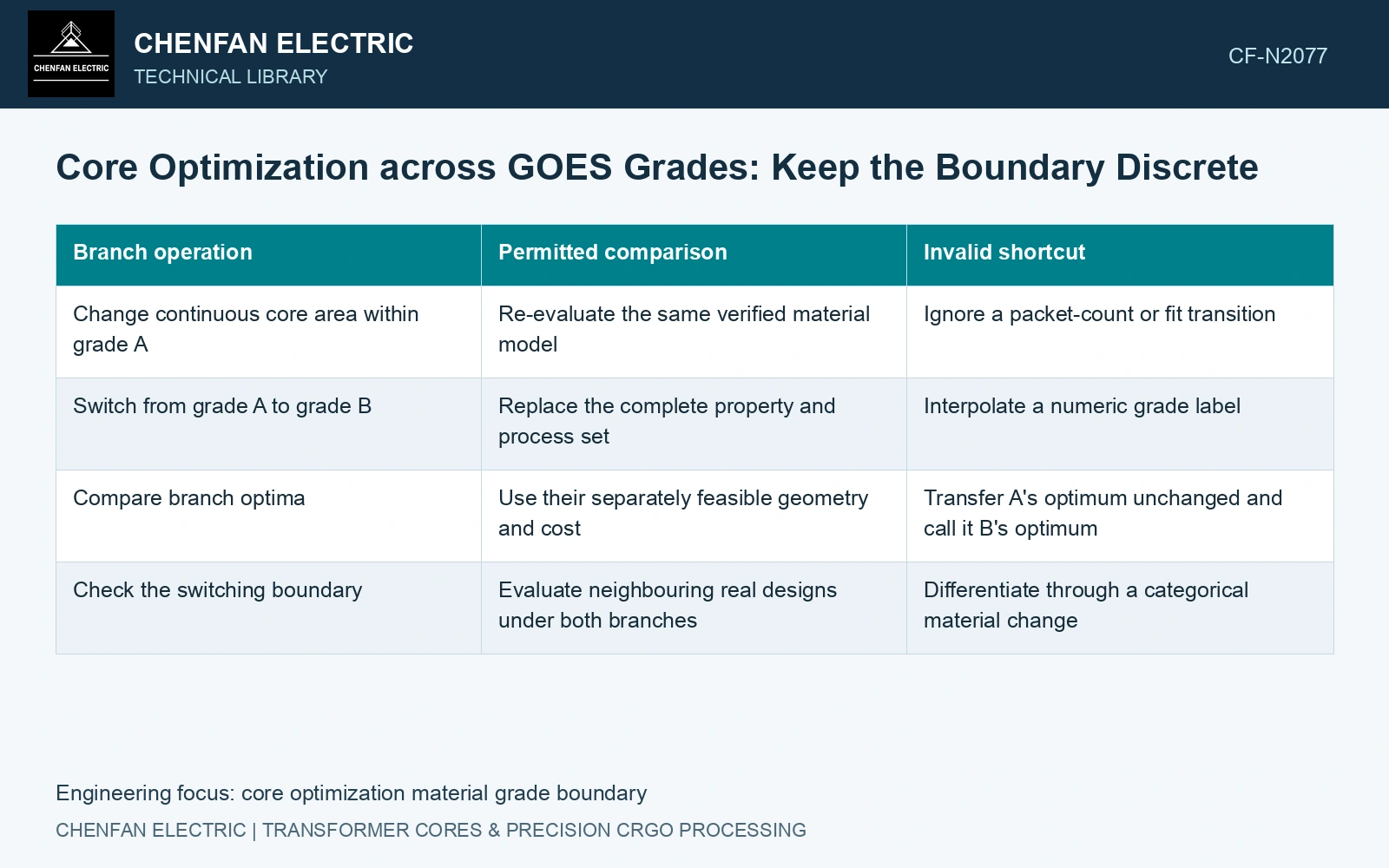
Build one coherent material branch at a time
Attach the grade’s gauge, coating, processing state and tested loss and magnetization data to its branch. A shared product-family name is not sufficient. Two grade options may require different available widths, heat-treatment restrictions or costs.
| Branch operation | Permitted comparison | Invalid shortcut |
|---|---|---|
| Change continuous core area within grade A | Re-evaluate the same verified material model | Ignore a packet-count or fit transition |
| Switch from grade A to grade B | Replace the complete property and process set | Interpolate a numeric grade label |
| Compare branch optima | Use their separately feasible geometry and cost | Transfer A’s optimum unchanged and call it B’s optimum |
| Check the switching boundary | Evaluate neighbouring real designs under both branches | Differentiate through a categorical material change |
Check derivatives where they actually exist
NIST response-surface methods address main effects, interactions and curvature within supported experimental coordinates [1]. Within a real grade branch, compare a proposed gradient with finite geometry perturbations at several sizes. Separate numerical remeshing noise from a physical response; a categorical grade change remains a separate branch.
Look for discontinuities from layer counts, duct layouts or constraint activation. A smooth loss function alone does not make the entire design problem smooth. At a branch boundary, report separate one-sided responses or enumerate the available choices rather than interpreting one derivative as the value of changing grade.
Map where real branches exchange preference
For a selected continuous design coordinate, plot the feasible grade-specific responses and identify where their objective ordering changes. Label regions where one grade fails a constraint, lacks material data or is unavailable in the required form. A curve crossing inside an unsupported region is not a usable switching point.
Then allow geometry to re-optimize within each surviving grade. The best section for one material can differ from that for another because loss, excitation and available gauge differ. Comparing both steels only at the first grade’s geometry can bias the result.
Compare actual catalogue branches at 1.7 T, 50 Hz: 23ZH90 at 0.90 W/kg and 23ZH85 at 0.85 W/kg, both 0.23 mm [2]. Assume steel masses of 1,000 kg and 1,040 kg. Ceiling-based strip budgets are 900 W and 884 W, only 16 W apart after the mass change. An assumed valuation of 8 currency units/W maps that budget difference to 128 currency units, but two independent maxima do not establish actual saved watts. Use paired assembled-core predictions or measurements with uncertainty before crediting a grade premium. Compare each purchasable grade at its own feasible geometry; do not invent an intermediate steel to smooth the economics.
Each material branch requires its own slit widths, coating state, cutting qualification and joint build. Retain those manufacturing identities throughout the optimisation and subsequent accepted-core comparison.
Issue the selected real grade, processing state and geometry together. List the design adjustments for alternative grades and reopen the affected branch calculations whenever material is substituted.
References
- NIST/SEMATECH, e-Handbook of Statistical Methods, Response surface designs, section 5.3.3.6.
- Nippon Steel Corporation, Grain-Oriented Electrical Steel Sheets, catalogue D004je, April 2020, specification and typical-property tables.