

Available strip widths turn a stepped-core optimum into a manufacturable packet schedule. Search the supported width set with slitting, coating and changeover costs visible beside magnetic section utilization.
Start the search with a dated width library. Identify which values are routinely supplied, which require a special slit, and which are excluded for the intended gauge and material. Availability of a parent coil does not establish availability of every finished lamination width.
Represent the actual packet schedule
Let wi be a permitted strip width, hi the total gross packet thickness assigned to that width across the section, and ki its applicable stacking factor. The approximate effective magnetic area is Σwihiki. Use consistent units and count mirrored packets once through their total thickness.
That area calculation is only one constraint. Locate each rectangle in the section and check its outer corners against the allowed envelope. For a circular envelope of radius R, a corner at transverse coordinates x,y must satisfy x² + y² ≤ R², before any required assembly allowance is deducted. A large area sum can still contain a protruding step.
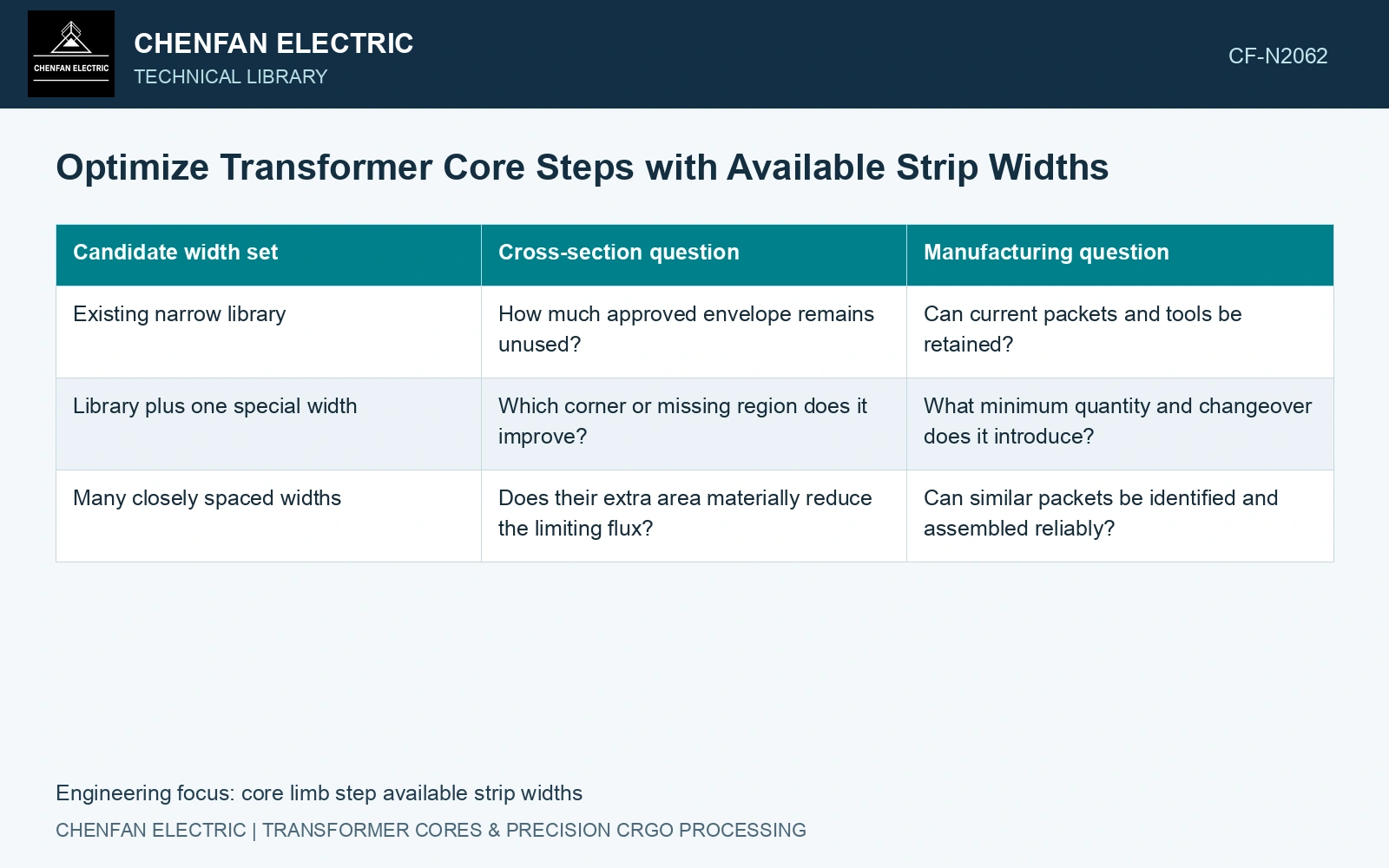
| Candidate width set | Cross-section question | Manufacturing question |
|---|---|---|
| Existing narrow library | How much approved envelope remains unused? | Can current packets and tools be retained? |
| Library plus one special width | Which corner or missing region does it improve? | What minimum quantity and changeover does it introduce? |
| Many closely spaced widths | Does their extra area materially reduce the limiting flux? | Can similar packets be identified and assembled reliably? |
Separate utilization from manufacturing complexity
Plot effective area divided by the agreed envelope area against the number of distinct packet variants. Show the actual width combinations beside the points. This makes a small geometric gain visible alongside its additional material identities, cutting programmes, storage positions and stacking transitions.
Packet thickness is discrete. Recheck integer counts and the measured gross thickness under the specified compression state; keep net steel and coating/contact space in separate ledgers.
Recalculate magnetic loading and loss for the chosen section, keeping joints, rolling direction and the relevant processing state consistent. A reduction in unused envelope does not establish lower assembled-core loss if it changes those features.
Use catalogue 0.23 mm nominal gauge [1], assumed here to represent net steel. Assume 100 central sheets at 200 mm width and two outer 100-sheet packets at 160 mm. Each packet has assumed measured gross thickness 24 mm, net steel 23 mm and stacking factor 23/24 = 0.95833. Net area is 200 × 23 + 160 × 46 = 11,960 mm²; multiplying this net account by another stacking factor would double count non-steel space. Replacing 160 by 170 mm gives 12,420 mm², a 3.85% gain. Assume a centred layout: central packet ends at y = ±12 mm; outer packets end at y = ±36 mm, within a permitted circle of radius 101 mm. Central and 170 mm outer corner radii are 100.72 and 92.31 mm. An assumed available 190 mm outer width instead reaches 101.59 mm and fails despite its larger area. At unchanged flux, a baseline 1.70 T becomes 1.70 × 11,960/12,420 = 1.637 T with 170 mm widths [2]. Advance that feasible geometric candidate for loss, joint and conversion-cost checks.
Permitted strip widths, integer sheet counts, coating build and compression determine the released schedule. Keep gross packet thickness distinct from the sum of nominal steel gauges in both drawings and calculation files.
Price each surviving width set per accepted core, including material yield, changeovers and handling. Compare the electrical gain of a special width with that complete conversion cost.
References
- Nippon Steel Corporation, Grain-Oriented Electrical Steel Sheets, catalogue D004je, April 2020, specification and typical-property tables.
- U.S. Department of Energy, DOE-HDBK-1011/4-92, Electrical Science, Volume 4, 1992.