

Converter-transformer current harmonics produce leakage fields in windings and nearby metal. A clamp or tank region can see a different harmonic mixture from another region. The terminal current spectrum is a model input; it is not a map of structural heat sources. Apply the HVDC transformer specification framework of IEC/IEEE 60076-57-129 to the stated liquid-immersed equipment [1].
Retain each harmonic’s magnitude, phase and distribution among windings. Transfer that set into the electromagnetic geometry, including screens, clamps and tank features. Compare calculated local field with material behavior before deciding whether independent harmonic solutions can be added.
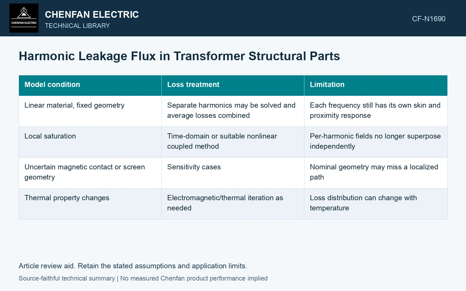
Know when frequency decomposition is valid
| Model condition | Loss treatment | Limitation |
|---|---|---|
| Linear material, fixed geometry | Separate harmonics may be solved and average losses combined | Each frequency still has its own skin and proximity response |
| Local saturation | Time-domain or suitable nonlinear coupled method | Per-harmonic fields no longer superpose independently |
| Uncertain magnetic contact or screen geometry | Sensitivity cases | Nominal geometry may miss a localized path |
| Thermal property changes | Electromagnetic/thermal iteration as needed | Loss distribution can change with temperature |
Phase matters before losses are calculated
At a structural location, fields from several windings combine vectorially. Adding their magnitudes instead of their complex contributions can overestimate or underestimate the local field. Conversely, a small total ampere-turn sum does not prove a small local leakage field when winding positions differ.
In a linear model, orthogonal frequencies can contribute separable time-average losses. This does not justify adding nonlinear loss results from isolated harmonic excitations when the combined waveform drives saturation. Identify the approximation in the report instead of calling both approaches “harmonic loss summation.”
Resolve local harmonic fields before adding heat
Assume two 250 Hz RMS field contributions at one structural location, 10 mT and 8 mT, opposing in phase. Their resultant is 2 mT; an aligned case gives 18 mT. Under an assumed linear local loss law proportional to B² at this fixed frequency, the aligned-to-opposed loss ratio is (18/2)² = 81. This illustrates why adding magnitudes before field solution can select the wrong hot region. Retain winding phase and geometry in the electromagnetic model, then verify whether its linear-material premise remains valid.
Connect the electromagnetic map to cooling
Export heat by structural region, with mesh and material assumptions, into the thermal model. A small total stray loss concentrated in a poorly cooled attachment can matter more locally than a larger distributed loss. Verify accessible temperatures at positions that correspond to the modelled regions.
If heating disagrees with the structural-loss map, check contacts, magnetic properties, harmonic phases and local cooling. Scaling all losses would obscure the specific hot path. Current distortion alone cannot assign a universal temperature penalty to that structure.
Include normal converter operation and converter-side faults in the transformer transient study [2].
References
- IEC/IEEE, IEC/IEEE 60076-57-129:2017, Power transformers – Part 57-129: Transformers for HVDC applications.
- CIGRE WG B4.51, Technical Brochure 609, Study of Converter Transients Imposed on the HVDC Converter Transformers, 2015.