

Dividing applied voltage by an average oil-gap width is a useful first description and a poor local acceptance criterion. A pressboard edge, overlap or nearby conducting feature can concentrate the field. Sustained DC can then redistribute voltage according to conductivity and charge history. Apply the HVDC transformer specification framework of IEC/IEEE 60076-57-129 to the stated liquid-immersed equipment [1]. [2]
Keep these mechanisms separate in the model. A geometric field concentration exists for a stated electrical boundary and material assignment. A later change in material conductivity or interfacial charge can move the field distribution even if the dimensions remain unchanged.
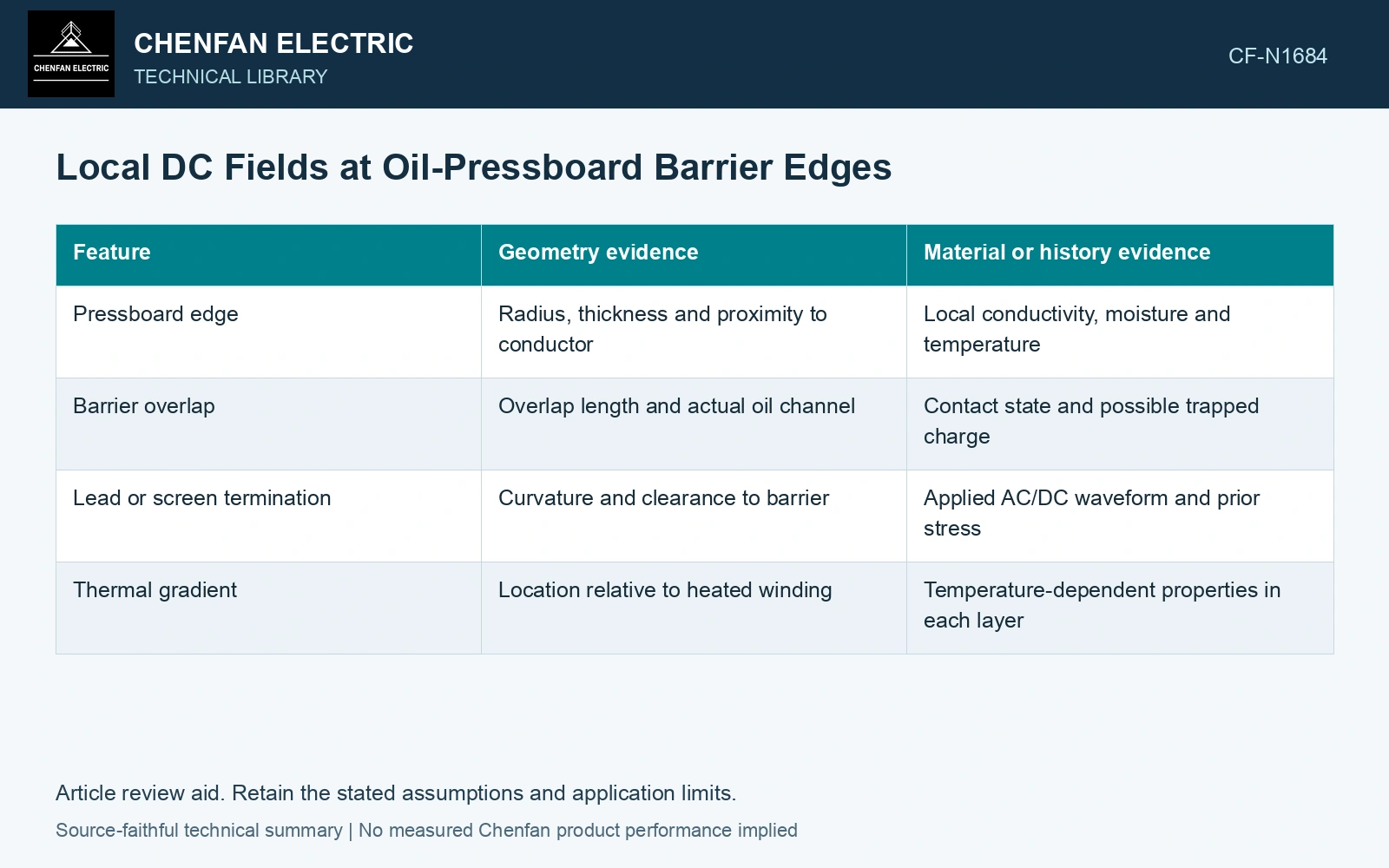
Inspect the path where the model predicts concentration
| Feature | Geometry evidence | Material or history evidence |
|---|---|---|
| Pressboard edge | Radius, thickness and proximity to conductor | Local conductivity, moisture and temperature |
| Barrier overlap | Overlap length and actual oil channel | Contact state and possible trapped charge |
| Lead or screen termination | Curvature and clearance to barrier | Applied AC/DC waveform and prior stress |
| Thermal gradient | Location relative to heated winding | Temperature-dependent properties in each layer |
Use a model ladder with clear boundaries
Begin with an electrostatic geometry calculation to locate sharp gradients for the stated permittivities. Then evaluate sustained DC using conductivity and the required time history. Where field-dependent conduction or charge transport matters, a stationary linear conduction solution is only a screening case.
In each model, examine a path across the oil gap and through the edge region. Record the local peak, the region over which it occurs and the numerical resolution. A peak at an ideal mathematically sharp edge can be mesh dependent; the manufactured radius and a suitable interpretation of field exposure are necessary.
Turn edge tolerances into a field sensitivity
Assume 200 kV across a 100 mm screening gap and a geometry-specific peak-to-average factor of 1.6: the local estimate is 1.6 × 200/100 = 3.2 kV/mm. An adverse 90 mm gap with assumed factor 1.8 gives 4.0 kV/mm, 25% higher. These factors are assumed model inputs, not material withstand values. Control the gap and manufactured edge radius represented by the adverse model, then obtain material and voltage-history evidence before making an acceptance decision.
Let dimensional inspection answer a field question
The useful inspection points follow the local-field mechanism: edge rounding, displaced barriers, overlap, burrs on nearby metal and compressed oil channels. An average winding-to-earth clearance may remain unchanged while one local path becomes smaller.
Compare the as-built tolerances with the modelled worst geometry. If the field solution uses a smooth radius but the drawing does not control it, the calculation and manufacturing evidence do not share the same premise. A defensible assessment reports that gap and obtains the missing geometry or verification rather than assigning a safe field from average voltage alone.
References
- IEC/IEEE, IEC/IEEE 60076-57-129:2017, Power transformers – Part 57-129: Transformers for HVDC applications.
- CIGRE JWG A2/B4.28, Technical Brochure 406, HVDC Converter Transformers – Design review, test procedures, ageing evaluation and reliability in service, 2010.