

The steel-price crossover shows when one core design becomes cheaper than another. Separate steel mass from conversion and material-condition costs to compare the choices over a usable purchasing range.
Compare credible price scenarios instead. Begin with designs that already meet the same technical duty and purchase requirements; an infeasible design does not become acceptable at a favourable price.
Separate the cost terms
For the independent common-grade purchase-cost model, let C = mp + F, where m is purchased steel allocated to the core, p its scenario price and F the design-dependent remainder. Define processing loss and scrap credit consistently. This is an initial-cost comparison; NIST’s cost framework separates acquisition from future operating costs, and its break-even method solves the input value at which alternatives tie. [1]
F can include cutting, stacking, treatment, tooling allocation and inspection, provided the accounting avoids double counting. If designs use different grades or processing routes, a single shared p is insufficient. Use separate price variables or an explicit premium relation.
Calculate the crossover
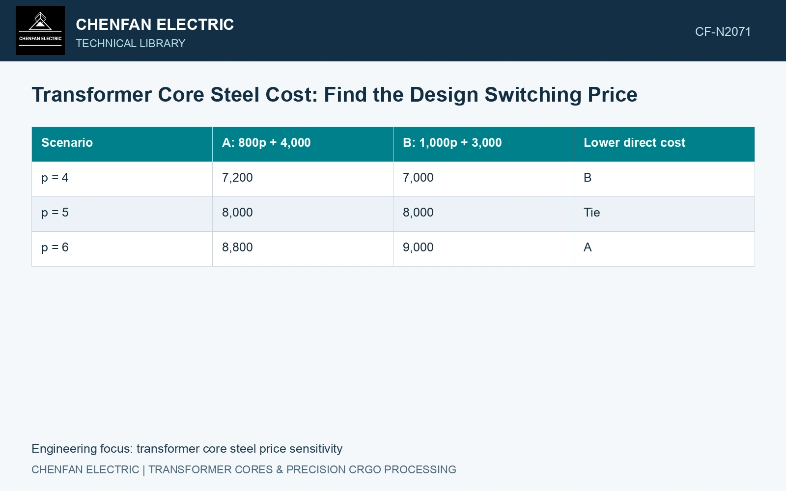
The following example uses fictional costs in an arbitrary currency. A uses 800 kg and has 4,000 of non-steel cost. B uses 1,000 kg and has 3,000 of non-steel cost. Assume an identical price p per kilogram and equal omitted costs.
| Scenario | A: 800p + 4,000 | B: 1,000p + 3,000 | Lower direct cost |
|---|---|---|---|
| p = 4 | 7,200 | 7,000 | B |
| p = 5 | 8,000 | 8,000 | Tie |
| p = 6 | 8,800 | 9,000 | A |
The switching price is (4,000 − 3,000)/(1,000 − 800) = 5 per kilogram. This is an algebraic threshold, not a prediction that steel will trade at that level. If both candidates have the same mass, their relative cost does not switch with a common steel price unless another price-dependent term differs.
Check which assumptions can move the threshold
A changed slit programme can alter purchased mass even when finished-core mass is fixed. A special coating, domain-refinement condition or gauge can change the grade premium and conversion route. Minimum order quantities and setup charges can make cost depend on batch size rather than on one core.
If operating loss differs, include its agreed present-value effect separately from initial steel cost [1]. State duty, study period, discounting and price basis. A steel-only crossover is not a complete life-cycle comparison.
Use the catalogue 7,650 kg/m³ density for two assumed feasible geometries: steel volumes 0.100 and 0.106 m³ give 765.0 and 810.9 kg. [2] Assume the second design reduces accepted-core loss by 40 W, valued at 8 currency units/W, and conversion costs are equal. The switching steel price is (40 × 8)/(810.9 − 765.0) = 6.97 currency units/kg. Below that price, the assumed loss value outweighs extra steel; above it, the lighter design has lower evaluated cost. Recompute the boundary with grade-specific prices and accepted-core losses; catalogue specific-loss ceilings alone do not supply the 40 W reduction.
Material yield, slit-width availability, joint schedule and conversion steps determine the purchased mass behind this boundary. Use input tonnes per accepted core rather than net magnetic steel alone when quotes include different conversion yields.
Compare the crossover with the credible purchasing range. Resolve the mass and conversion assumptions that move it most, giving procurement a design choice that remains clear across the relevant steel prices.
References
- J. Kneifel and D. Webb, NIST Handbook 135e2025, Life Cycle Costing Manual for the Federal Energy Management Program, August 2025, sections 4.2 and 8.3. DOI: 10.6028/NIST.HB.135e2025.
- Nippon Steel Corporation, Grain-Oriented Electrical Steel Sheets, catalogue D004je, April 2020, specification and typical-property tables.