

Sparse GOES curves define a bounded design search and a targeted test programme. Keep measured regions, interpolation and extrapolation distinct so a low predicted loss leads to the evidence needed for selection.
Before fitting a curve, map the evidence in induction and frequency, with separate maps for gauge, grade and processing state. A point measured in the rolling direction at a specified waveform belongs only to that condition.
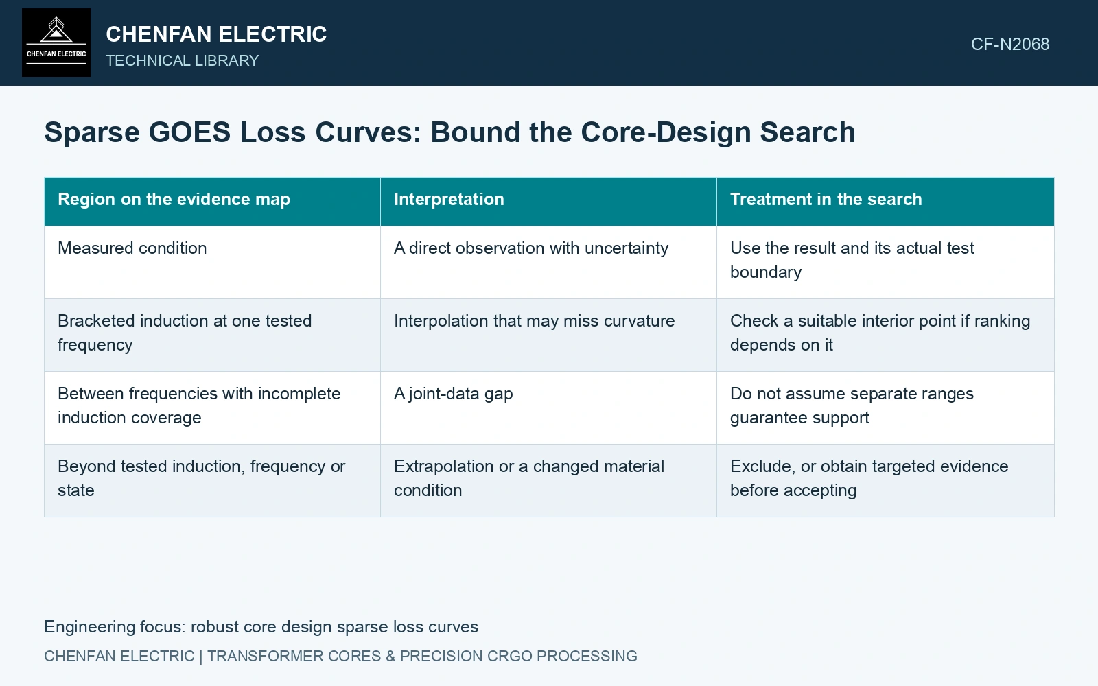
Classify the material domain
| Region on the evidence map | Interpretation | Treatment in the search |
|---|---|---|
| Measured condition | A direct observation with uncertainty | Use the result and its actual test boundary |
| Bracketed induction at one tested frequency | Interpolation that may miss curvature | Check a suitable interior point if ranking depends on it |
| Between frequencies with incomplete induction coverage | A joint-data gap | Do not assume separate ranges guarantee support |
| Beyond tested induction, frequency or state | Extrapolation or a changed material condition | Exclude, or obtain targeted evidence before accepting |
A rectangle formed from the lowest and highest values of each coordinate can contain combinations never tested. Even being inside a convex hull does not guarantee adequate local coverage when samples are widely separated or the response changes sharply. Show the actual points and gaps, not just the outer bounds.
Test the part of the curve that controls the decision
If competing designs operate at different inductions, a missing point near one candidate can dominate the ranking. Request measurements near that region, at the relevant frequency and processing state, rather than adding many points where both designs are already well supported.
Keep the curve physically coherent when testing pessimistic alternatives. Perturbing every coordinate independently can produce an implausible sequence or combine correlated measurement errors incorrectly. Use defensible whole-curve variants and distinguish material spread from instrument uncertainty.
A fitted loss model can interpolate efficiently, but its functional form is an assumption. Near saturation, waveform changes or a processing transition, a low-order fit may conceal a change in behaviour. Good agreement at the supplied points is insufficient because a highly flexible model can reproduce those points exactly while behaving badly between them. [1]
Compare designs under the uncertain curves
Re-evaluate each candidate under the supported central curve and the credible alternative bounds. Record whether feasibility or candidate order changes. Bounds chosen by engineering judgement should be labelled as scenarios; they are not measured confidence limits.
The 23ZH90 catalogue point is a maximum 0.90 W/kg at 1.7 T and 50 Hz. [2] Assume a search proposes 1.8 T, 50 Hz and applies a fitted power law p ∝ Bⁿ. Exponents assumed as 1.6 and 2.2 give 0.90(1.8/1.7)¹·⁶ = 0.986 W/kg and 0.90(1.8/1.7)²·² = 1.021 W/kg. For an assumed 1,000 kg steel inventory, that arbitrary modelling choice moves the budget by about 34.4 W. Neither result is a catalogue guarantee. Obtain a supported curve over the search region or constrain the candidate to covered conditions instead of allowing an unsupported exponent to decide the optimum.
Grade identity, rolling direction, stress relief and cutting state must match the fitted curve. A denser numerical interpolation cannot repair missing material measurements after a manufacturing change.
Use the decision map to specify missing induction, frequency, waveform and processing-state tests. Purchase the additional data that can change the design choice.
References
- NIST/SEMATECH, e-Handbook of Statistical Methods, Model Validation, section 4.4.4, and Estimation, section 4.1.3.1.
- Nippon Steel Corporation, Grain-Oriented Electrical Steel Sheets, catalogue D004je, April 2020, specification and typical-property tables.