

A multi-frequency core must satisfy the voltage programme and waveform at every required operating point. Compare each candidate across those excitation and loss cases, then identify the duty governing each constraint. [1]
Define each permitted operating case before assigning weights. Otherwise the optimizer can reduce average loss while leaving a short but mandatory duty outside its magnetic or thermal limits.
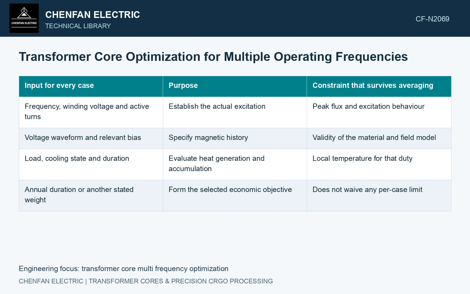
Construct a frequency-duty map
| Input for every case | Purpose | Constraint that survives averaging |
|---|---|---|
| Frequency, winding voltage and active turns | Establish the actual excitation | Peak flux and excitation behaviour |
| Voltage waveform and relevant bias | Specify magnetic history | Validity of the material and field model |
| Load, cooling state and duration | Evaluate heat generation and accumulation | Local temperature for that duty |
| Annual duration or another stated weight | Form the selected economic objective | Does not waive any per-case limit |
Using a constant voltage at a lower frequency raises sinusoidal flux for fixed turns and area. A controlled voltage/frequency programme can behave differently. Apply the actual programme, rather than assuming either relationship because it makes the candidate look favourable.
Separate energy preference from feasibility
Consider fictional loss predictions for two permitted cases lasting 6,000 and 1,000 hours annually. Candidate A loses 200 W and 350 W; B loses 230 W and 250 W. Their illustrative annual energies are 1,550 kWh and 1,630 kWh respectively. A wins this energy objective even though B has lower loss in the second case.
Neither result establishes acceptability. If A exceeds a local temperature or excitation limit in the second duty, its lower annual energy does not rescue it. If durations are uncertain, vary the weights and show where preference changes. Keep exceptional short-time cases as explicit checks instead of giving them a negligible annual weight and effectively deleting them.
Use data that cover the frequency and waveform
A single-frequency steel loss point cannot establish a reliable wide-frequency response. Verify that loss and magnetization data cover the candidate’s excitation range and test waveform. The selected model must also represent relevant induced-current and skin effects in conductors and structural parts as frequency changes.
Recompute thermal response where losses or cooling conditions change; fixed total watts do not establish a fixed hot spot. Assess electrical insulation and winding losses with their own applicable methods.
The catalogue’s 1.7 T, 50 Hz loss condition is an anchor, not a frequency conversion law. [2] Assume a candidate has 1.60 T at 50 Hz for one fixed winding voltage. At 60 Hz with unchanged turns and area, B becomes 1.60 × 50/60 = 1.333 T; at 45 Hz it becomes 1.778 T. The low-frequency case exceeds the catalogue induction point even though frequency itself is lower. Re-evaluate every permitted voltage/frequency pair with applicable loss and excitation data; neither constant B nor constant specific loss is justified by reusing the 50 Hz point.
Effective steel area, sheet count and joint build set the common physical design across frequencies. Lock those manufacturing inputs while evaluating each excitation case, then revise the whole design if the low-frequency corner fails.
Label the controlling case for every constraint on each candidate. It may be the lower-frequency magnetic case for one design and the higher-frequency loss case for another. That label is more useful than one “multi-frequency efficiency” figure, and it keeps the design decision tied to the duties the equipment must actually carry.
References
- U.S. Department of Energy, DOE-HDBK-1011/4-92, Electrical Science, Volume 4, 1992.
- Nippon Steel Corporation, Grain-Oriented Electrical Steel Sheets, catalogue D004je, April 2020, specification and typical-property tables.