

Multiwinding load combinations change the spatial source of leakage flux. Compare the shield across the specified power-transfer cases to locate the load state governing each local field and temperature limit. [1] [2]
Enumerate physically valid cases
Start from the transformer’s permitted winding duties and connections. Record currents, phase relationships, tap positions and the corresponding balance constraints. Do not combine independent maximum winding currents if that combination cannot occur in the specified electrical system.
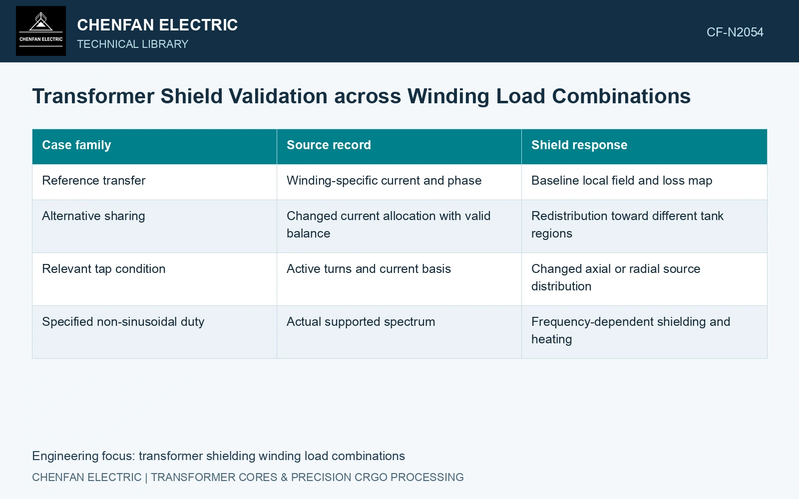
Distinguish normal rated transfer from alternative power sharing, operation of an auxiliary or tertiary winding and any specified imbalance or harmonic condition. Include a case only where the duty definition supports it. The table should identify the omitted combinations and why they are outside scope.
| Case family | Source record | Shield response |
|---|---|---|
| Reference transfer | Winding-specific current and phase | Baseline local field and loss map |
| Alternative sharing | Changed current allocation with valid balance | Redistribution toward different tank regions |
| Relevant tap condition | Active turns and current basis | Changed axial or radial source distribution |
| Specified non-sinusoidal duty | Actual supported spectrum | Frequency-dependent shielding and heating |
Recompute the spatial source
Use the actual winding locations and geometry for each current set. The winding-asymmetry paper shows that geometry influences the field reaching structural metal. An ampere-turn balance alone does not describe the complete spatial cancellation between separated winding regions. [2]
The multi-step shield method assumes a particular short-circuit-test source balance and simplified field-transfer stages. It should not be applied to another loading condition without checking those assumptions. Nonlinear shield loading can also prevent simple addition of separately solved field contributions.
Look for a different limiting region
Retain peak shunt density, tank and shield losses, and local temperatures for every supported case. Compare the locations of their maxima. One loading combination may govern the shunt end while another governs a lead-exit or a different tank wall.
Use the appropriate thermal duration and cooling condition from the duty specification. A transient high loss and a sustained lower loss can produce different temperature outcomes; a steady-state result cannot represent both automatically.
For an assumed linear teaching model, use referred RMS ampere-turn phasors (primary, secondary A, secondary B). Cases (100, −50, −50) and (100, −100, 0) both sum to zero and preserve primary input duty. Assume a particular tank point has signed transfer coefficients (0.003, 0.001, 0.003) T per referred ampere-turn, reflecting different winding positions. Local B is 0.10 T in the first case and 0.20 T in the second. At fixed frequency and geometry, an assumed P ∝ B² proxy gives four times the local indicator. Thus balanced total ampere-turns do not determine a local field. Include both valid power-sharing cases in qualification, then replace these fictional coefficients and linear loss proxy with the actual nonlinear field/thermal solution.
Acceptance should identify the case controlling each relevant limit and the uncertainty or margin associated with it. That makes a non-rated local maximum visible instead of hiding it behind a single total-load percentage.
References
- Z. Jurković, B. Jurišić and T. Župan, Multi-Step Approach for Fast Calculation of Magnetic Field in Transformer Tank Shields, Energies 17, 1378, 2024. DOI: 10.3390/en17061378.
- I. A. Hernandez-Robles et al., Analysing and Computing the Impact of Geometric Asymmetric Coils on Transformer Stray Losses, Applied System Innovation 7, 26, 2024. DOI: 10.3390/asi7020026.