

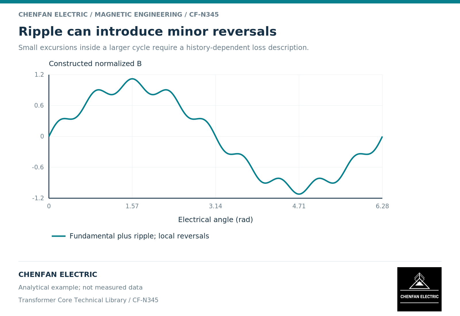
Ripple can create smaller magnetic reversals within a larger alternating excursion. These minor hysteresis loops may affect loss and current response even when the principal flux peak changes only slightly. A model that follows only the outer envelope can miss the history associated with those reversals.
Look for reversals in flux, not only ripple in voltage
Voltage ripple changes the slope of flux because induced voltage is proportional to dPhi/dt. A ripple component does not automatically reverse the flux trajectory; it must change the sign of the total relevant slope over an interval.
Integrate the complete induced waveform and inspect the resulting turning points. A high-frequency voltage component can alter local slope strongly while contributing a smaller flux amplitude because integration weights it by inverse frequency. This distinction helps separate a visibly rippled voltage from a genuinely nested magnetic excursion.
Basic magnetics guidance discusses minor loops under reduced or switched excitation. [1] The illustration is a physical mechanism, not a universal correction factor for utility-frequency core loss.
Preserve the order of the turning points
A minor loop is defined by its trajectory and reversal history. Two waveforms with the same minimum and maximum density can traverse different paths between them. Sorting measured data by density or retaining only extrema can destroy the information needed by a hysteresis model.
The useful record includes the time sequence, the larger-cycle operating region and the amplitude and duration of the smaller reversals. Bias and temperature should remain attached to the dataset when they affect the material response.
A conceptual diagram should show arrows through the nested loop. It should not imply that the loop is an isolated cycle if it is actually embedded in a changing major trajectory.
Match the loss method to the waveform
An explicit history-dependent model can track reversal behavior when its parameters are supported by relevant data. A loss formula may instead use an empirical treatment calibrated for particular waveform families. Neither approach is automatically valid for every ripple pattern.
Constitutive-model documentation distinguishes hysteretic models from single-valued magnetic relations. [2] A normal magnetization curve may support a field solution without containing the dissipative history needed for a minor-loop loss calculation.
Do not add a generic percentage to sinusoidal loss merely because ripple exists. The result depends on the trajectory, material, frequency content and the way dynamic loss contributions are represented. Any empirical correction should identify its source, calibration range and validation evidence.
Build a reversal-aware validation record
| Quantity | Why it is retained |
|---|---|
| Main flux trajectory | Defines the operating region of each small reversal |
| Reversal times and levels | Defines the minor-loop history |
| Excitation rate | Supports rate-dependent loss treatment |
| Material and direction | Establishes the constitutive boundary |
| Independent waveform case | Tests prediction beyond the fitting data |
For an assembled core, local field direction and joint behavior may differ from a uniform material specimen. A specimen model should therefore be evaluated within the assembly model rather than promoted directly into a complete-core loss guarantee.
The engineering outcome should identify whether ripple materially changes the relevant loss or current result and how that conclusion was checked. A larger number of modeled loops is not inherently better; the model must have data that support their behavior. This keeps the analysis focused on the actual waveform rather than on visually impressive but unvalidated hysteresis plots.
References
[1] Lloyd Dixon / Texas Instruments. Magnetics Design 1 – Introduction and Basic Magnetics.
[2] Cesare Tozzo / COMSOL. Modeling Ferromagnetic Materials in COMSOL Multiphysics.