

Remanence and closing angle act together in an inrush calculation. The closing angle determines the subsequent voltage integral; residual flux supplies the initial offset. Their signs can reinforce or oppose each other. Neither input, considered alone, determines the resulting current peak.
Write the initial condition into the flux equation
Consider an illustrative ideal winding with induced voltage e(t) = E_m sin(omega t + theta), applied at t = 0. With N turns and initial flux Phi_r, integration gives:
Phi(t) = Phi_r + E_m/(omega N) [cos(theta) – cos(omega t + theta)].
Here E_m is peak induced voltage, omega is angular frequency and theta is the phase angle at closing. This follows directly from the voltage-flux relationship. [1] It neglects winding drops, source impedance, hysteretic feedback and any pole-to-pole switching sequence, so it is an excitation illustration rather than a complete inrush model.
The offset term is Phi_r + E_m cos(theta)/(omega N). This is why residual polarity and closing angle cannot be specified independently of the same reference convention.
Compare two limiting illustrations carefully
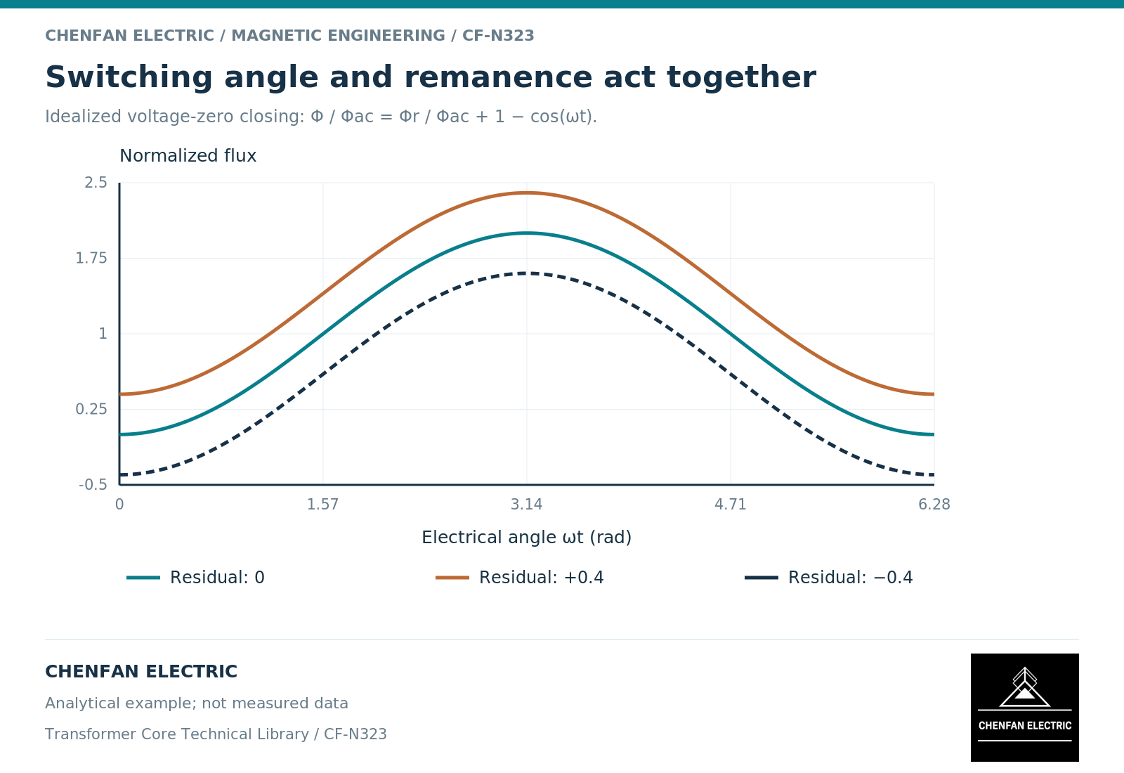
Let the centered sinusoidal flux amplitude E_m/(omega N) be 1.0 per unit. At a positive-going voltage zero, theta = 0, an initially zero-flux ideal winding reaches a flux excursion of 2.0 per unit during the first half-cycle. With an initial flux of +0.4 per unit, the same ideal expression reaches 2.4 per unit; with -0.4, it reaches 1.6.
At a voltage peak, theta = pi/2, the voltage-driven offset term is zero. A nonzero residual state still shifts the waveform, however. Closing at a particular angle is therefore not a universal guarantee of a centered flux trajectory.
These values are mathematical examples, not allowable flux densities or predictions of a transformer’s current. The actual circuit responds when the core enters a strongly nonlinear region, modifying the induced voltage through its impedance drops.
Current requires the nonlinear circuit
To calculate inrush current, the model must connect flux linkage to magnetizing current and include the external and winding circuits. The high-field characteristic, leakage representation and source impedance affect the response. Classical saturation-model documentation explicitly discusses limitations associated with branch placement and unavailable deep-saturation data. [2]
A steep rise in current does not mean flux has increased in the same proportion. Near saturation, a relatively small additional flux excursion can require a large increase in magnetizing ampere-turns. Do not convert the ideal 2.4 per-unit flux example into a current multiple by a linear ratio.
For a three-phase transformer, switching times and magnetic coupling add another layer. The residual states must be compatible with the topology rather than assigned as three unrelated favorable values.
Build a joint sensitivity study
Vary closing angle, residual state and circuit conditions together over the relevant range. Report the state assumptions alongside each result. A study that fixes remanence to zero while varying only angle may miss the controlling case; a study that selects the largest independent residual in every branch may create an impossible state.
Keep measured breaker timing information separate from ideal command angles. Also distinguish a predicted statistical distribution from a small set of deterministic sensitivity cases.
The engineering result should identify the combinations that control the chosen observable and the evidence supporting those combinations. It should not reduce a coupled transient problem to a slogan such as “close at voltage peak” or a single residual-flux percentage.
References
[1] Lloyd Dixon / Texas Instruments. Magnetics Design 1 – Introduction and Basic Magnetics.
[2] Manitoba Hydro International / PSCAD. The Classical Approach.