

A magnetic probe near a lamination edge may report a small component normal to the sheet. That signal can indicate a real three-dimensional field, but it can also arise when a much larger in-plane component leaks into the normal channel through misalignment or cross-talk.
Define the quantity before selecting the probe. A sensor outside the sheet measures a local field at its sensing volume. It does not directly report the magnetization vector inside the steel. Inferring an internal component needs additional geometry and a justified field model.
Set a component coordinate system
Mark rolling direction, transverse direction and the sheet normal. Record the probe’s axes and the transformation into that system. Verify alignment under the actual mounting arrangement, including any change in standoff or surface tilt during scanning.
Calibrate or check cross-axis response in suitable known fields. A datasheet’s sensitivity for one axis does not establish the assembled probe’s ability to resolve a small component beside a large orthogonal field.
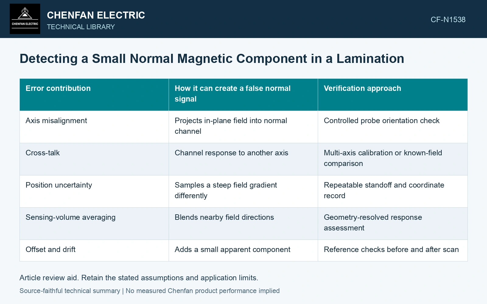
| Error contribution | How it can create a false normal signal | Verification approach |
|---|---|---|
| Axis misalignment | Projects in-plane field into normal channel | Controlled probe orientation check |
| Cross-talk | Channel response to another axis | Multi-axis calibration or known-field comparison |
| Position uncertainty | Samples a steep field gradient differently | Repeatable standoff and coordinate record |
| Sensing-volume averaging | Blends nearby field directions | Geometry-resolved response assessment |
| Offset and drift | Adds a small apparent component | Reference checks before and after scan |
The error budget should be compared with the component being interpreted, rather than only with the largest measured field.
Use geometry as a discriminating check
Repeat a suitable reference measurement after a controlled probe rotation or reversal, accounting for the expected component transformation. A real vector component and a fixed sensor offset transform differently. The experiment should preserve position closely enough that moving in a steep gradient does not obscure the comparison.
Map edges, overlaps and joint regions with their actual geometry. A normal component near an edge does not demonstrate the same field throughout a packet. Accessible surface measurements may also miss an internal path.
Connect the measured pattern to the model
Compare component directions and spatial distributions, not only magnitudes. The specified wound-core research abstract reports interlaminar flux effects in its particular inner/outer-core boundary; it does not establish a universal pattern for every stacked core. Use topology-specific evidence.
A model used to infer internal magnetization should reproduce the external measurement with the probe’s spatial averaging included where significant. Different internal distributions may produce similar accessible fields, so the inference can remain nonunique.
Report the demonstrated resolution of the normal component, the accessible region and unresolved model assumptions. The resulting map is useful when the normal signal exceeds the identified error contributions and follows a physically consistent pattern. A colorful three-axis plot without that error budget may merely display an amplified projection of the dominant in-plane field.
Technical references
- Materials / MDPI. Magnetostrictive Properties of the Grain-Oriented Silicon Steel Sheet under DC-Biased and Multisinusoidal Magnetizations.
- NIST. NCAL: Diffraction Stress Measurement Under Applied Load.
- IEEJ / J-STAGE. Influence of Interlaminar Flux between Cores on Iron Loss in Three-legged Wound Transformer Core.