

The relay sees a favorable angle and issues a command. While the breaker mechanism moves, the motor bus continues to slip relative to the alternate source. The relevant angle is the one at contact closure, not the earlier measured value. [1]
Prediction needs the relative frequency and its change over the delay. A fixed frequency difference may be adequate locally, but nonlinear motor rundown can invalidate it as the bus decays.
Define the sign before calculating
Let δ be bus angle minus source angle, in radians. Let Δf be bus frequency minus source frequency, in hertz. Then dδ/dt = 2πΔf. If a = d(Δf)/dt is approximately constant over closing delay τ, the predicted angle is δpred = δ0 + 2πΔf0τ + πaτ². Time τ is in seconds and a is in hertz per second.
This is a local kinematic approximation. It assumes valid estimates and a sufficiently short interval for the stated acceleration model. It is not an approved relay setting or a guarantee of safe reconnection.
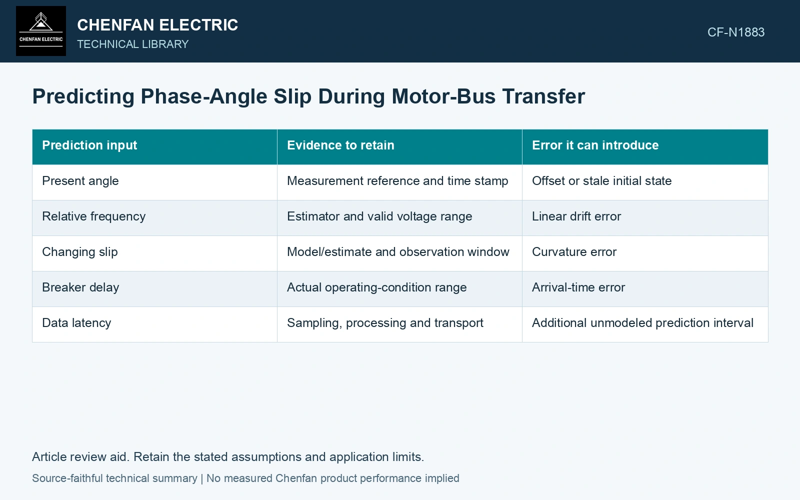
| Prediction input | Evidence to retain | Error it can introduce |
|---|---|---|
| Present angle | Measurement reference and time stamp | Offset or stale initial state |
| Relative frequency | Estimator and valid voltage range | Linear drift error |
| Changing slip | Model/estimate and observation window | Curvature error |
| Breaker delay | Actual operating-condition range | Arrival-time error |
| Data latency | Sampling, processing and transport | Additional unmodeled prediction interval |
Include the age of the estimate
A phasor result represents a measurement window, not an instantaneous point free of delay. Establish its effective time reference and include processing and communication latency where relevant. Otherwise the prediction can begin from a state that is already older than the assumed τ.
The SEL transfer paper discusses predicting angle over closing time and blocking excessive changing-slip conditions. Its specific implementation does not establish the estimator accuracy of another relay or installation.
Propagate a range, not one perfect point
Evaluate credible ranges for slip, acceleration and delay. Where their errors are correlated, do not combine them using an independence assumption without evidence. A conservative envelope may be more appropriate than a narrow statistical band.
Compare predicted arrival-angle ranges with actual recorded closure where such evidence exists. Retain unsuccessful predictions as well as favorable events; they reveal conditions in which the local model loses validity.
Record whether each estimator or timing uncertainty is a bound or a standard uncertainty before combining it. Sensitivity and correlation affect a combined uncertainty; they must match the selected arrival-angle model. [2]
Include changing slip in closure prediction
Assume initial relative angle 10°, relative frequency −2 Hz, frequency acceleration −5 Hz/s and delay 0.050 s. Arrival angle is 10 + 360(−2)(0.050) + 180(−5)(0.050²) = −28.25°. Constant-slip prediction gives −26°, differing by 2.25°. Compare the whole credible delay range before accepting the local approximation.
References
- P. Muralimanohar, D. Haas, J. R. McClanahan, R. T. Jagaduri and S. Singletary, Implementation of a Microprocessor-Based Motor Bus Transfer Scheme, IEEE PCIC, 2016, DOI: 10.1109/PCICON.2016.7589248.
- B. N. Taylor and C. E. Kuyatt, NIST Technical Note 1297, Guidelines for Evaluating and Expressing the Uncertainty of NIST Measurement Results, 1994, sections 5 and 6.