

A transfer model labels several loads pumps and gives them one speed-squared torque curve. That can be a useful approximation in a qualified case, but the process condition matters. Valve position, fluid behavior, check mechanisms and mechanical friction can change what the motor must overcome. [1]
The load model should answer a concrete question: what resisting torque acts at each speed during the disturbance and recovery? Rated shaft power supplies one operating point, not the whole answer.
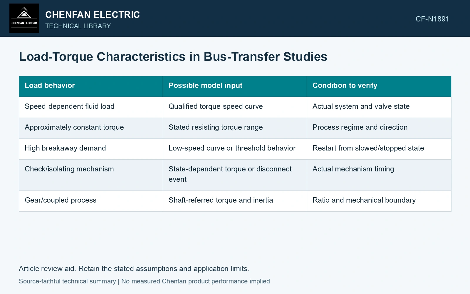
Select a curve with a stated domain
For a simplified aerodynamic or centrifugal load under appropriate fixed conditions, torque may be represented as TL = kω². TL is in newton-metres, ω is angular speed in radians per second and k has units consistent with that relation. The coefficient and valid range need evidence.
| Load behavior | Possible model input | Condition to verify |
|---|---|---|
| Speed-dependent fluid load | Qualified torque-speed curve | Actual system and valve state |
| Approximately constant torque | Stated resisting torque range | Process regime and direction |
| High breakaway demand | Low-speed curve or threshold behavior | Restart from slowed/stopped state |
| Check/isolating mechanism | State-dependent torque or disconnect event | Actual mechanism timing |
| Gear/coupled process | Shaft-referred torque and inertia | Ratio and mechanical boundary |
The table is a model-selection map. It does not assign any actual machine to a category without its data.
Keep inertia outside the torque curve
Inertia determines how net torque changes speed. It is not another resisting torque to be added arbitrarily. Use J dω/dt = Te − TL with both torques referred to the same shaft and a valid representation of the coupled load.
A high-inertia load can preserve speed during interruption yet require longer recovery. A low-inertia load can slow rapidly but recover quickly if sufficient torque exists. These outcomes cannot be inferred from rated power alone.
Compare margin through the vulnerable speeds
Plot electrical and load torque across the relevant dynamic trajectory. The source voltage and machine state affect electrical torque. A positive margin near rated speed does not prove that the machine can pass a lower-speed region where the load curve changes.
The SEL transfer paper uses manufacturer-provided motor information and a specified load-torque model. That evidence supports validation of the chosen curve, not reuse of its particular curve for an unrelated process.
At a defined slip, reduced supply voltage can reduce induction-motor torque approximately with voltage squared; the load torque and inertia still determine acceleration. [2]
Compare load torque at reduced speed
Assume a fan has 100 N·m load torque at rated speed and follows a speed-squared law over the range examined. At 0.8 pu speed its load torque is 64 N·m; an assumed constant-torque machine still needs 100 N·m. Compare available motor torque with each curve, rather than assigning identical recovery to equal rated kW.
References
- P. Muralimanohar, D. Haas, J. R. McClanahan, R. T. Jagaduri and S. Singletary, Implementation of a Microprocessor-Based Motor Bus Transfer Scheme, IEEE PCIC, 2016, DOI: 10.1109/PCICON.2016.7589248.
- J. Rees, M. Kjellberg and S. Kling, ABB, Softstarter Handbook, 1SFC132060M0201, November 2010.