

The laser-refinement benefit curve shows how a GOES grade performs across the transformer’s excitation range. Measure paired loss and excitation at the relevant inductions to connect material selection with actual duty.
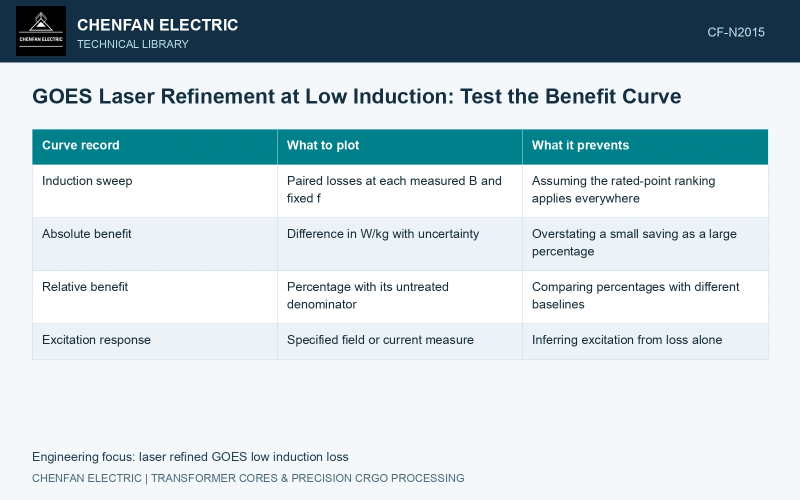
Plot paired differences over the excitation range
Use treated and untreated specimens matched for parent material, gauge, orientation and processing. At each selected induction B and frequency f, record their specific losses under the same test conditions. Define the absolute benefit as p untreated − p refined, in W/kg. A positive value indicates lower loss in the refined specimen.
Show the percentage benefit separately as 100 times that difference divided by the untreated loss. At low induction, a small absolute difference can produce an apparently large percentage when the denominator is small. Its engineering importance and uncertainty therefore need to remain visible.
| Curve record | What to plot | What it prevents |
|---|---|---|
| Induction sweep | Paired losses at each measured B and fixed f | Assuming the rated-point ranking applies everywhere |
| Absolute benefit | Difference in W/kg with uncertainty | Overstating a small saving as a large percentage |
| Relative benefit | Percentage with its untreated denominator | Comparing percentages with different baselines |
| Excitation response | Specified field or current measure | Inferring excitation from loss alone |
Separate measured behaviour from a loss explanation
Domain refinement changes the magnetic reversal process, but a low-induction loss difference is not a direct measurement of one loss component. Hysteresis, classical eddy-current and excess-loss descriptions require appropriate measurements and a model with stated assumptions. A single-frequency sweep does not uniquely separate those contributions. [1]
The laser study reports specimen results at its stated conditions and gives no universal low-induction benefit curve [1]. Manufacturer specifications use stated preparation and measurement points; a maximum is not an interpolation rule [2].
Check the resolution where the signal becomes small
At low excitation, instrument offsets, waveform control and specimen repeatability may become more prominent relative to the measured power. Use the laboratory’s uncertainty evaluation at each point rather than applying a fixed percentage from the rated test. Repeat measurements after the same magnetic preparation, and report points where the paired difference cannot be distinguished from uncertainty.
The 23ZH90 ≤0.90 W/kg point is at 1.7 T, 50 Hz, not a low-induction curve [2]. Assume matched 0.5 T, 50 Hz losses 0.070/0.066 W/kg: saving 0.004 W/kg, or 5.71%, equals only 4 W for assumed 1,000 kg. With paired expanded uncertainty ±0.006 W/kg, its interval −0.002 to +0.010 includes zero [3]. Do not credit a confirmed low-induction benefit. Retain absolute differences, improve discrimination and measure the required duty range before monetizing treatment.
Treatment pitch, stress state, coating and cut history must be matched at each induction point. Do not combine the low-induction strip result with a different assembled-core joint or clamping state.
Select the comparison range from the intended duty. If the economic calculation uses annual no-load energy, apply the measured or justified curve to the actual operating distribution. A rated-point saving is useful evidence for that point; it becomes a duty-wide saving only after the remaining excitation range has been addressed.
References
- P. Rauscher et al., The influence of laser scribing on magnetic domain formation in grain oriented electrical steel visualized by directional neutron dark-field imaging, Scientific Reports 6, 38307, 2016, Table 1. DOI: 10.1038/srep38307.
- Nippon Steel Corporation, Grain-Oriented Electrical Steel Sheets, catalogue D004je, April 2020, specification and typical-property tables.
- B. N. Taylor and C. E. Kuyatt, NIST Technical Note 1297, Guidelines for Evaluating and Expressing the Uncertainty of NIST Measurement Results, 1994, sections 5 and 6.