

Joint limb-and-yoke optimization asks where added steel changes the limiting magnetic region. Compare paired effective sections and joints, charging each change for its material and space.
Treat limb and yoke areas as paired design choices. Their relationship follows the magnetic topology and construction, rather than a rule that both must be equal.
Identify the limiting magnetic region
SEL’s transformer fundamentals describe how core construction changes the magnetic return paths [1]. For each duty, establish the flux in the actual limb and yoke segments. Do not assign equal flux merely from drawing symmetry; preserve connections and the number of available return paths.
The ratio Φ/A gives an average flux-density screen using the appropriate effective magnetic area. Joints introduce local transfer between laminations, gaps and directions. Their peaks, excitation demand and loss cannot be established by dividing the limb flux by the largest gross yoke rectangle.
Use separate outputs for the straight limb, straight yoke and limiting joint region. Where a simplified magnetic model is retained, make the joint correction and its validation range visible. The geometry used in a loss estimate should match the candidate’s actual overlap and packet schedule.
Evaluate four paired changes
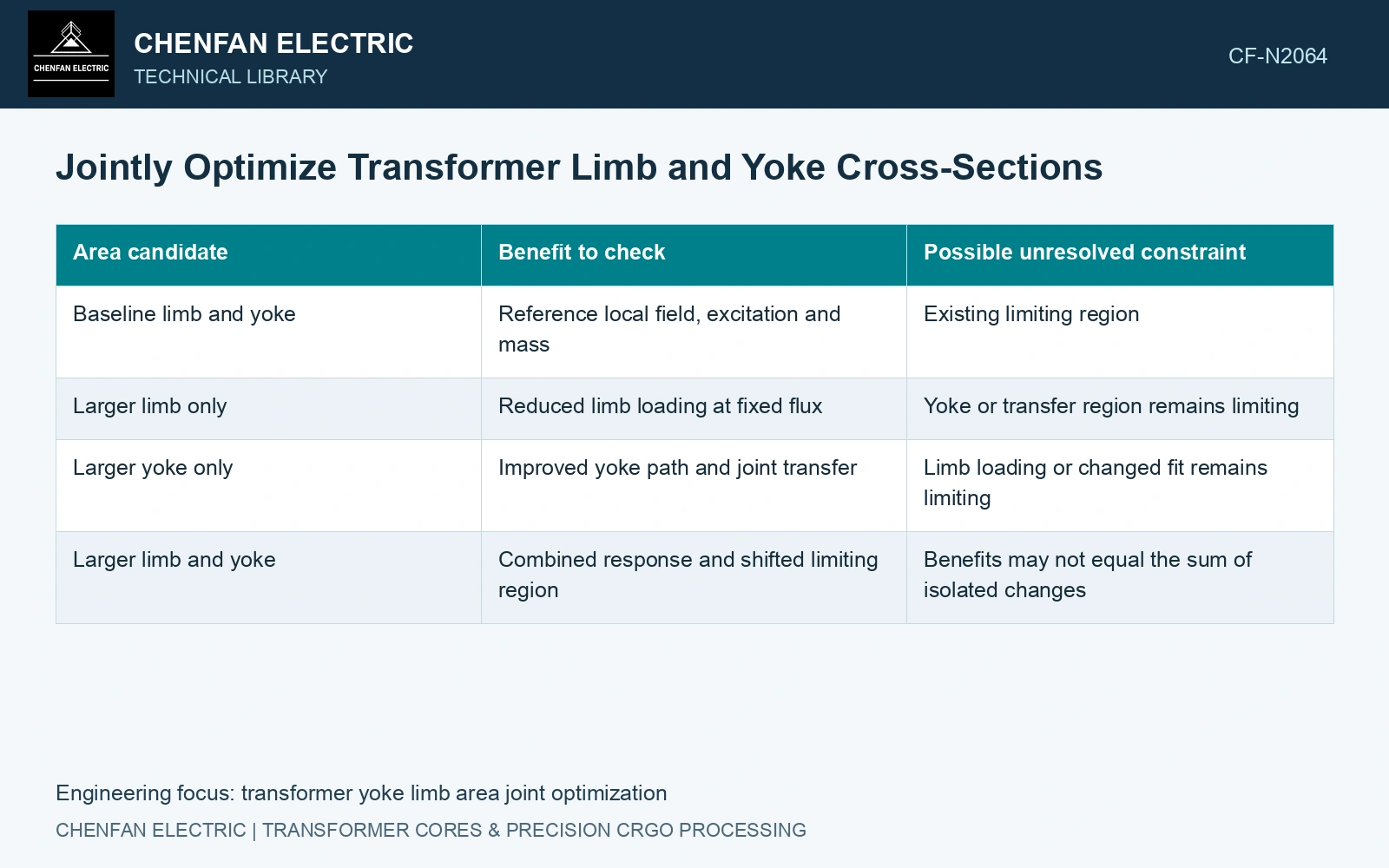
| Area candidate | Benefit to check | Possible unresolved constraint |
|---|---|---|
| Baseline limb and yoke | Reference local field, excitation and mass | Existing limiting region |
| Larger limb only | Reduced limb loading at fixed flux | Yoke or transfer region remains limiting |
| Larger yoke only | Improved yoke path and joint transfer | Limb loading or changed fit remains limiting |
| Larger limb and yoke | Combined response and shifted limiting region | Benefits may not equal the sum of isolated changes |
This is a comparison matrix, not a predicted ranking. Recalculate the magnetic solution at every point. Local redistribution can change the benefit of the second addition, especially near nonlinear material response or a revised overlap geometry.
Charge each change for its real material and space
For unchanged straight-segment length, the approximate incremental steel mass is density × total segment length × added net steel cross-section. Use the sum of all affected lengths. If enlarging the yoke moves coil clearances, corner geometry or the core envelope, rebuild those regions instead of applying the straight-segment estimate to the whole assembly.
Compare the additional mass with the change in the limiting performance output, and retain the other constraints: excitation current, loss, coil fit and temperature. A small reduction in average flux may be irrelevant if a local joint still controls the design.
The catalogue density of 7,650 kg/m³ prices a section change physically. [2] Assume total affected straight-yoke length 2.0 m and additional net steel section 0.0010 m²: added steel mass is 15.3 kg. If assumed yoke flux is 0.016 Wb and its net section rises from 0.010 to 0.011 m², mean yoke induction falls from 1.60 to 1.455 T. That 0.145 T reduction belongs only to the stated return-path section. If the limb remains at its assumed limiting 1.70 T, enlarging the yoke has not removed the limb constraint. Re-evaluate the joint and paired sections before buying the additional steel.
Limb and yoke width schedules, rolling direction, corner overlap and clamp registration determine where flux transfers. Manufacture the selected pair as one controlled construction rather than independently optimising two rectangles.
Issue the selected limb and yoke packet schedules with their effective-area basis. Show which return-path or joint constraint justifies each section and its material cost.
References
- B. Kasztenny, M. Thompson and N. Fischer, Schweitzer Engineering Laboratories, Fundamentals of Short-Circuit Protection for Transformers, 2012 revision.
- Nippon Steel Corporation, Grain-Oriented Electrical Steel Sheets, catalogue D004je, April 2020, specification and typical-property tables.