

Grading shields manage electric stress, while their ends introduce local geometric boundaries. ABB discusses field-control shielding in instrument insulation [1]. Use the actual CT primary/secondary architecture rather than importing a generic bushing section.
Intermediate shields and their ends must be assessed in the actual primary-insulation and secondary-lead architecture. A generic bushing section does not define the CT’s local electrical boundary.
Locate each end in three dimensions
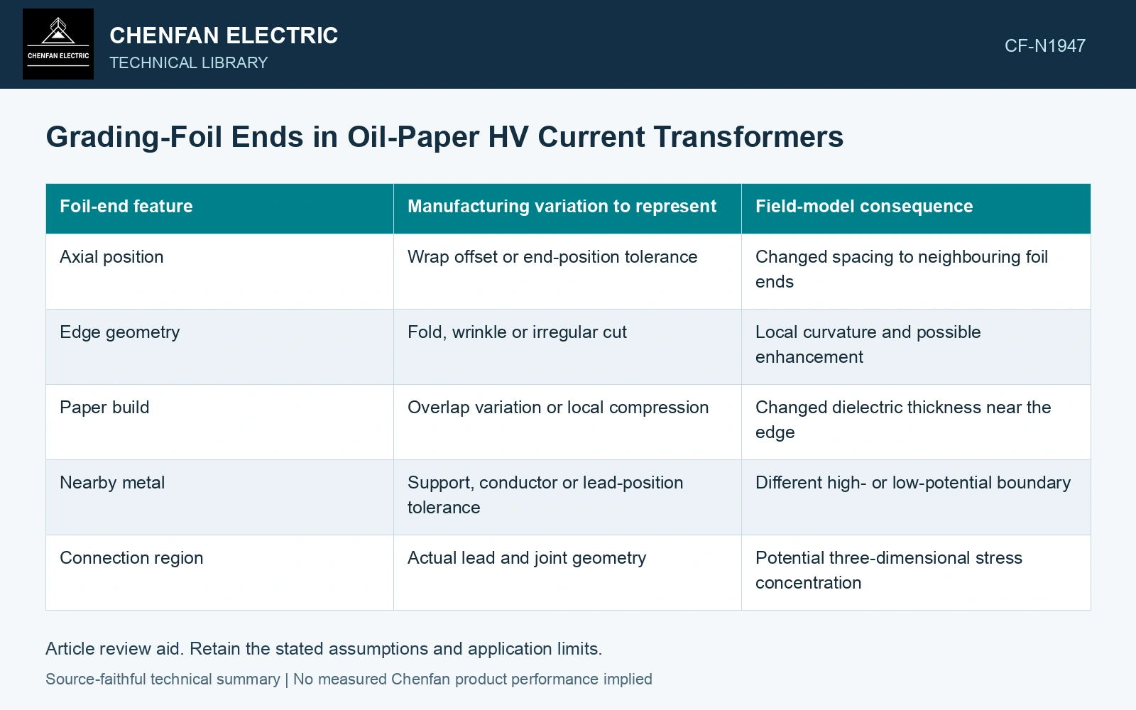
Retain axial end position, edge shape and circumferential features such as overlaps or connections. Add the local paper thickness and nearby metal. A foil length alone does not determine the nearest electrical boundary; a displaced winding or support can change that boundary without changing the foil itself.
| Foil-end feature | Manufacturing variation to represent | Field-model consequence |
|---|---|---|
| Axial position | Wrap offset or end-position tolerance | Changed spacing to neighbouring foil ends |
| Edge geometry | Fold, wrinkle or irregular cut | Local curvature and possible enhancement |
| Paper build | Overlap variation or local compression | Changed dielectric thickness near the edge |
| Nearby metal | Support, conductor or lead-position tolerance | Different high- or low-potential boundary |
| Connection region | Actual lead and joint geometry | Potential three-dimensional stress concentration |
Use voltage difference on the right pair of boundaries
For a defined approximately planar region, Eavg = ΔV/d in V/m, consistent with the capacitor potential difference [2]. This is an author’s geometric screen, not the curved foil-end peak. The full field needs assigned potentials, dielectric properties and actual edge/nearby-metal geometry.
Floating grading layers acquire potentials from the surrounding capacitive system. If a connection or neighbouring geometry changes, their voltages may change as well. Do not hold every foil at its nominal potential while independently moving the geometry unless that approximation is justified.
Compare plausible tolerance combinations
Start with the nominal assembly, then examine combinations that reduce the relevant separation or sharpen an edge. Combining every unrelated maximum tolerance may create an impossible assembly, while considering one tolerance at a time can miss a credible joint displacement. Use the manufacturing constraint relationships to choose the cases.
Identify where an axisymmetric model is valid. A local fold, connection tab or secondary lead exit may require a three-dimensional model. Mesh convergence matters at the end: an apparent peak tied to a coarse or singular idealized edge needs interpretation rather than blind comparison.
Assume ΔV = 10 kV across 10 mm: Eavg = 1 kV/mm. Fictional edge factors 2/4 give local screens 2/4 kV/mm. Against an assumed 3 kV/mm review cap, one passes and the other fails despite equal average voltage division. Hold the second layout and replace the factors with a resolved field solution using real radii, folds and paper build. These factors/cap are neither measured results nor dielectric-strength limits. A smooth mean-potential plot cannot qualify a foil end.
Translate the result into identifiable inspection features: which end positions, paper sections and neighbouring parts control the acceptable geometry. That gives production staff something specific to verify and prevents a correctly counted foil stack from being mistaken for a correctly manufactured field-grading system.
References
- ABB, Instrument Transformers: Technical Information and Application Guide, 1VAP420003-TG, revision A, December 2004.
- U.S. Department of Energy, DOE-HDBK-1011/2-92, Electrical Science, Volume 2, 1992.