

A planar 2D Cartesian reactor-gap model assumes translational invariance in the omitted direction; an axisymmetric model instead assumes rotational symmetry. A real finite-width packet lets flux spread around its ends, so a centre-plane solution cannot automatically represent the whole gap or end heating. [1]
Name the direction omitted by the 2D model and measure the actual packet width. Identify nearby winding, clamps and end structures that can intercept fringing flux. The need for a 3D correction depends on the result being used: total inductance, local field or metal heating.
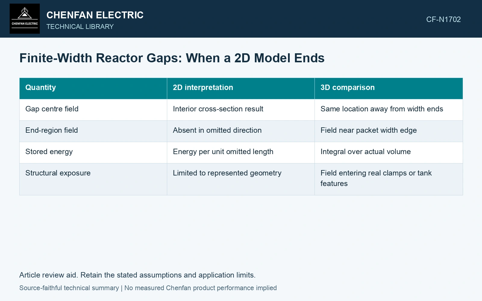
Compare quantities with matching definitions
| Quantity | 2D interpretation | 3D comparison |
|---|---|---|
| Gap centre field | Interior cross-section result | Same location away from width ends |
| End-region field | Absent in omitted direction | Field near packet width edge |
| Stored energy | Energy per unit omitted length | Integral over actual volume |
| Structural exposure | Limited to represented geometry | Field entering real clamps or tank features |
Choose a submodel boundary that preserves the field
A local 3D gap submodel needs boundary conditions representative of the full magnetic circuit. Moving the boundary too close can artificially confine fringing. Extend the region and compare until the result used for the decision is stable within a stated tolerance.
Keep material data, current and gap geometry consistent between models. Compare the centre section first; a large mismatch there may indicate different assumptions rather than end effects. Then inspect the region the 2D model cannot represent.
Propagate the uncertainty of the decision quantity, including justified input/model contributions. Agreement at one centre point alone supplies no uncertainty bound for the omitted end region. [2]
Compare centre and end model quantities
Assumptions: at the same 50 Hz peak-current state, the 2D centre field is 1.00 T, the 3D centre is 1.02 T and the 3D end is 1.25 T. Centre disagreement is 2%, within an assumed 3% agreement screen. But a separately justified end-field standard uncertainty of 0.03 T gives a k = 2 lower bound of 1.19 T, exceeding an assumed 1.10 T local ceiling by 0.09 T. Reject the 2D model for that end-region decision. The 3D prediction still needs independent field/thermal validation; centre agreement cannot establish it. [1] [2]
Extrapolate only what was tested
For design review, show the 2D centre result, the 3D centre result and the 3D end result on the same excitation basis. Report how much each decision-relevant quantity changes. This supports a justified simplification where it works and identifies the end region that still needs three-dimensional treatment.
References
- H. B. Duc, T. P. Minh, T. P. Anh and V. D. Quoc, A Novel Approach for the Modeling of Electromagnetic Forces in Air-Gap Shunt Reactors, Engineering, Technology & Applied Science Research 12, 8223–8227, 2022. DOI: 10.48084/etasr.4692.
- B. N. Taylor and C. E. Kuyatt, NIST Technical Note 1297, Guidelines for Evaluating and Expressing the Uncertainty of NIST Measurement Results, 1994, sections 5 and 6.